
Resolving Focal Depth with Near-Field Single Station in Sparse Seismic Networks
Accurate resolution of focal depth is vital for seismic hazard assessments and studies of seismogenesis. This study investigates a near-field seismic depth phase called sPL, which is generated by S-waves reflected as P-waves at the free surface. Unlike traditional methods utilizing P and S arrival times, sPL allows for reliable focal depth determination from a single station within sparse seismic networks. We illustrate its application using aftershock sequences from the 2013 Lushan and 2011 Virginia earthquakes, demonstrating that sPL enables effective depth resolution by analyzing differential times between P and sPL phases.

Resolving Focal Depth with Near-Field Single Station in Sparse Seismic Networks
E N D
Presentation Transcript
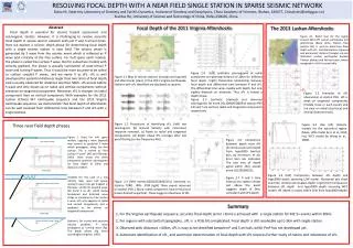
RESOLVING FOCAL DEPTH WITH A NEAR FIELD SINGLE STATION IN SPARSE SEISMIC NETWORK Sidao Ni, State Key Laboratory of Geodesy and Earth’s Dynamics, Institute of Geodesy and Geophysics, China Academy of Sciences, Wuhan, 430077, China(sdni@whigg.ac.cn) Xiaohui He, University of Science and Technology of China, Hefei,230026, China Abstract Focal depth is essential for seismic hazard assessment and seismogenic studies. However, it is challenging to resolve accurate focal depth in sparse seismic network with just P and S arrival times. Here we explore a seismic depth phase for determining focal depth with a single seismic station in near field. The seismic phase is generated by S wave from the seismic event which is reflected as P wave post-critically at the free surface. For half space earth models, the phase is called free surface P wave. But for subsurface models with velocity gradient, the phase is actually summation of post-critical P wave and turning P waves. Thus it would be more accurate to be called as surface coupled P waves, and we name it as sPL. sPL is well developed for epicentral distances larger than two times of focal depth, and is usually observed for distances less than 50km. sPL arrives before S wave and only shows up on radial and vertical components without presence on tangential component. Moreover, sPL is stronger on radial component than on vertical component. With examples for the 2013 Lushan (China) M7 earthquake sequence and the 2011 Virgina earthquake sequence, we demonstrate that focal depth of aftershocks can be well resolved from differential time between P and sPL with a single stations. Focal Depth of the 2011 Virginia Aftershocks The 2013 Lushan Aftershocks Figure 3.1. Relief map for the region around 2013 M7 Lushan earthquake and aftershocks (black dots). Station TQU (yellow dot) is used to determine focal depth with sPL. Portable stations (squares) and permanant stations (triangle) are also indicated. Lushan earthquake borders Tibetan plateau and Sichuan basin, where topographic relief is remarkable. Figure 2.4 (left) Synthetic seismograms of radial component at epicentral distance of 20km for different focal depth. (right) theoretical relationship between focal depth and differential time between P and sPL. The differential time varies rapidly with depth, but only slightly depends on distances. Thus sPL is indeed a depth phase. Figure 2.5 Synthetic (dashed) and observed seismograms for event 20110830034828 at station IP05. Z,R and T are vertical, radial and tangential components respectively Figure 2.1 Map of seismic stations (triangle and squares) and aftershocks (stars) of the 2011 Virginia Earthquake. Stations with sPL identified are displayed as squares. sPL Figure 3.2 Examples of sPL observation at station TQU. sPL is weak on tangential components (middle trace in each panel) and are clear on radial (top trace) and vertical (bottom trace). Figure 2.2 Procedures of identifying sPL. (left) raw seismogram. (b) Ground Velocity with instrument response removed. (c) Roate to radial and tangential components. (d) Depth phase sPL emerges after low pass filtering (corner frequency 4Hz). Figure 3.3 (top left) Velocity models for the epicentral region (black, LZW model by Li et al, 2013; red, WCY model by Wang et al., 2000). Three near field depth phases Figure 1. (top) For half space models, upgoing s wave (dashed) may convert to postcrital P wave which propagates along the free surface. This is named as “free surface P wave” (Aki and Richards, 2002). Inset shows the three component synthetic seismograms for focal depth of 10km and distance of 40km. (middle) For the case of a low velocity layer upon half space, upoing S wave may get trapped in the layer, and forms coupled wave. We name it as sPL, which shows broadened and distorted wave shape as compared to free surface P wave. sPL only appears on radial and vertical components, and is expected to be absent on tangential components. (bottom). For crustal with poisitive velocity gradient, P wave propagates as turning wave (Pg). The depth phase sPg forms accordingly (Langston, 1987). Figure 2.6 Comparison between depth from sPL (horizontal axis) and depth from hypo2000 (vertical axis, by Herrmann et al). Error bars are indicated. The two sets of depth agree within 1km, except event 201203260321. Figure 2.7 P and S time interval at a station almost just above the event suggests depth of 3km, consistent with sPL depth. Free Surface P wave Time (sec) Figure 3.4 (left) Comparison between sPL depth and hypo2000 depth assuming LZW model. Horizontal axis show event No. Vertical axis displays depth. (right) Com Comparison between sPL depth and hypo2000 depth assuming WCY model. sPL depth is mostly within 3km from hypo2000 depths. Figure 2.3 (left) event13(20120326032151) observed on stations CVRD、IP05、IP04 (right) Three events observed on station IP05. ( Black: radial component, blue vertical and brown dashed tangential). These suggest robustness of sPL. Upgoing S surface coupled wave sPL Summary 1, For the Virginia earthquake sequence, accurate focal depth (error <1km) is achieved with a single station for M2.5+ events within 30km. 2, For regions with substantial topography , sPL is a little bit complicated. Focal depth is still resolvable up to 3km with single station. 3, Observed with distances < 60km, sPL is easy to be identified between P and S arrivals, while PmP has not developed yet. 4, Automatic identification of sPL, and automatic determination of focal depth with sPL requires further study of nature and robustness of sPL. Time (sec) Surface reflected turning P wave sPg


