Download
1 / 46
490 likes | 607 Views
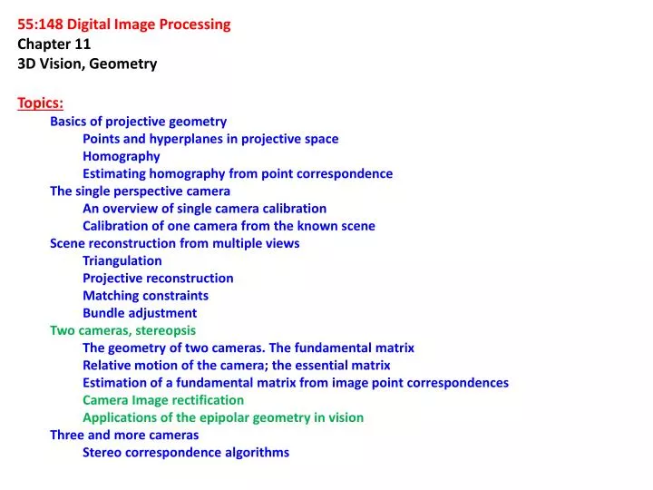
55:148 Digital Image Processing Chapter 11 3D Vision, Geometry Topics: Basics of projective geometry Points and hyperplanes in projective space Homography Estimating homography from point correspondence The single perspective camera An overview of single camera calibration

E N D
55:148 Digital Image Processing • Chapter 11 3D Vision, Geometry • Topics: • Basics of projective geometry • Points and hyperplanes in projective space • Homography • Estimating homography from point correspondence • The single perspective camera • An overview of single camera calibration • Calibration of one camera from the known scene • Scene reconstruction from multiple views • Triangulation • Projective reconstruction • Matching constraints • Bundle adjustment • Two cameras, stereopsis • The geometry of two cameras. The fundamental matrix • Relative motion of the camera; the essential matrix • Estimation of a fundamental matrix from image point correspondences • Camera Image rectification • Applications of the epipolar geometry in vision • Three and more cameras • Stereo correspondence algorithms
Image epipolar rectification • Illustrative description • Both image planes being coplanar • Baseline along the horizontal axis (x-axis) of the image plane • Two epipoles at infinity along the horizontal direction • Horizontal epipolar lines Before After
Image epipolar rectification • Illustrative description • Both image planes being coplanar • Baseline along the horizontal axis (x-axis) of the image plane • Two epipoles at infinity along the horizontal direction • Horizontal epipolar lines • Method: Apply suitable homographic transformation on each image Before After
Image rectification • Analytic description • Suppose that we know camera matrices and for the two cameras • The objective is to rotate each image planes around their optical centers until their focal planes becomes coplanar • Thereby, containing the baseline • More specifically, the new x-axis is parallel to the baseline • Both images have y-axis x-axis • Thus, new camera matrices
Image rectification • Analytic description • Suppose that we know camera matrices and for the two cameras • The objective is to rotate each image planes around their optical centers until their focal planes becomes coplanar • Thereby, containing the baseline • More specifically, the new x-axis is parallel to the baseline • Both images have y-axis x-axis • Thus, new camera matrices • where,
Image rectification • Analytic description • Suppose that we know camera matrices and for the two cameras • The objective is to rotate each image planes around their optical centers until their focal planes becomes coplanar • Thereby, containing the baseline • More specifically, the new x-axis is parallel to the baseline • Both images have y-axis x-axis • Thus, new camera matrices • where, • The new x-axis is parallel to the baseline
Image rectification • Analytic description • Suppose that we know camera matrices and for the two cameras • The objective is to rotate each image planes around their optical centers until their focal planes becomes coplanar • Thereby, containing the baseline • More specifically, the new x-axis is parallel to the baseline • Both images have y-axis x-axis • Thus, new camera matrices • where, • The new x-axis is parallel to the baseline • The new y-axis is orthogonal to the new x-axis , for some and
Image rectification • Analytic description • Suppose that we know camera matrices and for the two cameras • The objective is to rotate each image planes around their optical centers until their focal planes becomes coplanar • Thereby, containing the baseline • More specifically, the new x-axis is parallel to the baseline • Both images have y-axis x-axis • Thus, new camera matrices • where, • The new x-axis is parallel to the baseline • The new y-axis is orthogonal to the new x-axis , for some and • The new z-axis is orthogonal to the new xy-plane
A proof that Image rectification a suitable homographic transformation
A proof that Image rectification a suitable homographic transformation Let For any 3D scene point , projected image points using camera matrices are:
A proof that Image rectification a suitable homographic transformation Let For any 3D scene point , projected image points using camera matrices are: Using the relation in homogeneous coordinate system,
A proof that Image rectification a suitable homographic transformation Let For any 3D scene point , projected image points using camera matrices are: Using the relation in homogeneous coordinate system,
A proof that Image rectification a suitable homographic transformation Let For any 3D scene point , projected image points using camera matrices are: Using the relation in homogeneous coordinate system, i.e.,
A proof that Image rectification a suitable homographic transformation Let For any 3D scene point , projected image points using camera matrices are: Using the relation in homogeneous coordinate system, i.e., : scale factor : 3-by-3 matrix ≈ perspective transformation ≈ homography equivalent HENCE PROVED
Image rectification • Algorithmic description • As we have seen from analytic discussionGiven the knowledge of and , image rectification process is precisely defined So, the first task is to determine camera matrices and • Algorithm Compute camera matrices and • Task 1: Solve using corresponding point pairs in two images and algebraic error minimization • Input: A linear system:
Image rectification • Algorithmic description • As we have seen from analytic discussionGiven the knowledge of and , image rectification process is precisely defined So, the first task is to determine camera matrices and • Algorithm Compute camera matrices and • Task 1: Solve using corresponding point pairs in two images and algebraic error minimization • Input: A linear system: • Using Kroneckerproduct identity: , we get
Image rectification • Algorithmic description • As we have seen from analytic discussionGiven the knowledge of and , image rectification process is precisely defined So, the first task is to determine camera matrices and • Algorithm Compute camera matrices and • Task 1: Solve using corresponding point pairs in two images and algebraic error minimization • Input: A linear system: • Using Kroneckerproduct identity: , we get • Put together all correspondences
Image rectification • Algorithmic description • As we have seen from analytic discussionGiven the knowledge of and , image rectification process is precisely defined So, the first task is to determine camera matrices and • Algorithm Compute camera matrices and • Task 1: Solve using corresponding point pairs in two images and algebraic error minimization • Input: A linear system: • Using Kroneckerproduct identity: , we get • Put together all correspondences • Compute and apply singular value decomposition; choose along the eigenvector corresponding to the smallest eigenvalue
Image rectification • Algorithmic description • As we have seen from analytic discussionGiven the knowledge of and , image rectification process is precisely defined So, the first task is to determine camera matrices and • Algorithm Compute camera matrices and • Task 1: Solve using corresponding point pairs in two images and algebraic error minimization • Input: A linear system: • Using Kroneckerproduct identity: , we get • Put together all correspondences • Compute and apply singular value decomposition; choose along the eigenvector corresponding to the smallest eigenvalue • For to be a valid fundamental matrix, its rank must be 2; but it may not satisfy in reality (why?); thus needs correction
Image rectification • Algorithmic description • As we have seen from analytic discussionGiven the knowledge of and , image rectification process is precisely defined So, the first task is to determine camera matrices and • Algorithm Compute camera matrices and • Task 1: Solve using corresponding point pairs in two images and algebraic error minimization • Input: A linear system: • Using Kroneckerproduct identity: , we get • Put together all correspondences • Compute and apply singular value decomposition; choose along the eigenvector corresponding to the smallest eigenvalue • For to be a valid fundamental matrix, its rank must be 2; but it may not satisfy in reality (why?); thus needs correction • SVD decomposition: ; set the smallest eigenvalue of to zero giving a new diagonal matrix ; use the new matrix
Image rectification • Algorithmic description • As we have seen from analytic discussionGiven the knowledge of and , image rectification process is precisely defined So, the first task is to determine camera matrices and • Algorithm Compute camera matrices and • Task 1: Solve using corresponding point pairs in two images and algebraic error minimization • Input: A linear system: • Using Kroneckerproduct identity: , we get • Put together all correspondences • Compute and apply singular value decomposition; choose along the eigenvector corresponding to the smallest eigenvalue • For to be a valid fundamental matrix, its rank must be 2; but it may not satisfy in reality (why?); thus needs correction • SVD decomposition: ; set the smallest eigenvalue of to zero giving a new diagonal matrix ; use the new matrix Note that ML estimation method incorporate the validity condition of F into the optimization process
Image rectification • Algorithmic description • As we have seen from analytic discussionGiven the knowledge of and , image rectification process is precisely defined So, the first task is to determine camera matrices and • Algorithm Compute camera matrices and • Task 1: Solve using corresponding point pairs in two images and algebraic error minimization • Input: A linear system: • Output: Fundamental matrix • Task 2: Decompose the fundamental to matrix camera matrices
Image rectification • Algorithmic description • As we have seen from analytic discussionGiven the knowledge of and , image rectification process is precisely defined So, the first task is to determine camera matrices and • Algorithm Compute camera matrices and • Task 1: Solve using corresponding point pairs in two images and algebraic error minimization • Input: A linear system: • Output: Fundamental matrix • Task 2: Decompose the fundamental to matrix camera matrices
Image rectification • Algorithmic description • As we have seen from analytic discussionGiven the knowledge of and , image rectification process is precisely defined So, the first task is to determine camera matrices and • Algorithm Compute camera matrices and • Task 1: Solve using corresponding point pairs in two images and algebraic error minimization • Input: A linear system: • Output: Fundamental matrix • Task 2: Decompose the fundamental to matrix camera matrices • Input of the algorithm : A linear system: • Output of the algorithm: camera matrices and
Image rectification • Algorithmic description • As we have seen from analytic discussionGiven the knowledge of and , image rectification process is precisely defined So, the first task is to determine camera matrices and • Algorithm Compute camera matrices and • Task 1: Solve using corresponding point pairs in two images and algebraic error minimization • Input: A linear system: • Output: Fundamental matrix • Task 2: Decompose the fundamental to matrix camera matrices • Input of the algorithm : A linear system: • Output of the algorithm: camera matrices and • Now what?
Image rectification Algorithmic description Algorithm Compute image rectification
Image rectification Algorithmic description Algorithm Compute image rectification Input: and Output: and and two homography transformations: and
Image rectification Algorithmic description Algorithm Compute image rectification Input: and Output: and and two homography transformations: and Decompose each camera matrices: and
Image rectification Algorithmic description Algorithm Compute image rectification Input: and Output: and and two homography transformations: and Decompose each camera matrices: and Determine two optical centers and using and and their decompositions
Image rectification Algorithmic description Algorithm Compute image rectification Input: and Output: and and two homography transformations: and Decompose each camera matrices: and Determine two optical centers and using and and their decompositions Determine new rotation matrix common to and
Image rectification Algorithmic description Algorithm Compute image rectification Input: and Output: and and two homography transformations: and Decompose each camera matrices: and Determine two optical centers and using and and their decompositions Determine new rotation matrix common to and Determine new intrinsic parameters by averaging and and then annulling skew component
Image rectification Algorithmic description Algorithm Compute image rectification Input: and Output: and and two homography transformations: and Decompose each camera matrices: and Determine two optical centers and using and and their decompositions Determine new rotation matrix common to and Determine new intrinsic parameters by averaging and and then annulling skew component Compute new projection matrices:
Image rectification Algorithmic description Algorithm Compute image rectification Input: and Output: and and two homography transformations: and Decompose each camera matrices: and Determine two optical centers and using and and their decompositions Determine new rotation matrix common to and Determine new intrinsic parameters by averaging and and then annulling skew component Compute new projection matrices: and
Image rectification Algorithmic description Algorithm Compute image rectification Input: and Output: and and two homography transformations: and Decompose each camera matrices: and Determine two optical centers and using and and their decompositions Determine new rotation matrix common to and Determine new intrinsic parameters by averaging and and then annulling skew component Compute new projection matrices: and Compute homography transformations
Image rectification Algorithmic description Algorithm Compute image rectification Input: and Output: and and two homography transformations: and Decompose each camera matrices: and Determine two optical centers and using and and their decompositions Determine new rotation matrix common to and Determine new intrinsic parameters by averaging and and then annulling skew component Compute new projection matrices: and Compute homography transformations and
Image rectification: application 3D reconstruction becomes easier b a c
Elementary stereo geometry in the rectified image configuration The depth of a 3D scene point can be calculated using the disparity measure
Elementary stereo geometry in the rectified image configuration The depth of a 3D scene point can be calculated using the disparity measure
Elementary stereo geometry in the rectified image configuration The depth of a 3D scene point can be calculated using the disparity measure
Elementary stereo geometry in the rectified image configuration The depth of a 3D scene point can be calculated using the disparity measure