TIME SERIES: MODELLING
TIME SERIES: MODELLING. IDENTIFICATION. Stationary?. MANIPULATE. M O D E L I N G. DIAGNOSTICS. REVISED. F O R E C A S T. E V A L U A T E. Stages in Modeling. No. Yes. arma. arima. NOT GOOD. Assumptions.

TIME SERIES: MODELLING
E N D
Presentation Transcript
IDENTIFICATION Stationary? MANIPULATE M O D E L I N G DIAGNOSTICS REVISED F O R E C A S T E V A L U A T E Stages in Modeling No Yes arma arima NOT GOOD
Assumptions • Building models based on past realizations of a time series we implicitly assume that there is some regularity in the process generating the series. • We view as if the series is produced by a specially designed “machine.” We attempt to find this machine. • Precondition. One way to view such regularity is through the concept of stationarity.
IDENTIFICATION Stationary? MANIPULATE M O D E L I N G DIAGNOSTICS REVISED F O R E C A S T E V A L U A T E IDENTIFICATION NO NOT GOOD
Check for Stationarity • A time series is covariance stationary if, for all values of t,
A time series is covariance stationary if its statistical properties do not change with time. • A stationary series = the mean and variance are constant across time and the covariance between current and lagged values of the series (autocovariances) depends only on the distance between the time points.
Stationary Time Series? • Stationary Process
Stationary Time Series? • Non-stationary Variance
Interpretation • We try to predict the future in terms of what has already been known. • And for the stationary series • But these two properties don't help very much to talk about the future.
Interpretation • More useful. That is, if g1 > 0, a ‘high’ value of Y today will likely be followed by a ‘high’ value tomorrow. • By assuming that the gk are stable, this information can be exploited and estimated.
Autocorrelations • Covariances are difficult to interpret, since they depend on the units of measurement. • Correlations are scale-free. Thus we can obtain the same information about the time series by computing the autocorrelations of a time series.
Autocorrelation Coefficient • The autocorrelation coefficient between Yt and Yt-k is • A graph of the autocorrelations is called a correlogram. • Knowledge of the correlogram implies knowledge of the process [model] which generated the series and vice versa.
Partial Autocorrelations • Another important function in analyzing time series is the partial autocorrelation function. • Partial autocorrelations measure the strength of the relationship between observations in a series controlling for the effect of intervening time periods.
If the observations of Y in period t are highly related to the observations in, say, period t-12, then a plot of the partial autocorrelations for that series (partial correlogram) should exhibit a ‘spike,’ or relative peak, at lag 12. • Monthly time series with a seasonal component should exhibit such a pattern in their partial correlograms. • Monthly time series with seasonal components will also exhibit ‘spikes’ in their correlograms at multiples of 12 lags.
Autocorrelations Partial Autocorrelations
IDENTIFICATION Stationary? MANIPULATE M O D E L I N G DIAGNOSTICS REVISED F O R E C A S T E V A L U A T E MODELING: ARMA NO NOT GOOD
Time Series Models • Two basic models commonly used: • Autoregressive model • Moving Average model • When you know the underlying process governing a time series you can remove its effect.
Autoregressive Processes (AR) • Regress variable on lags of itself only • univariate process • How many lags? • look at t-stats • how smooth is data • AR(1): Yt = 0+ 1Yt-1 + εt
Autoregressive Process of order p, AR(p) : • Note how mechanical the model is—no attempt to explain Y other than to say it follow its past history • lag length arbitrary Yt = 0+ 1Yt-1 + 2Yt-2 +...+ pYt-p + εt
AR(1): Yt = f0 + f1 Yt-1 + et f1 = .9 Note: smooth long swings away from mean
AR(1): Yt = f0 + f1 Yt-1 + et f1 = .9 Note: exponential decay
AR(2): Yt = 0 + f1 Yt-1 + f2 Yt-2 + et f1 = 1.4, f2 = -.45 Note: smooth long swings away from mean
AR(2): Yt = f0 + f1 Yt-1 + f2 Yt-2 + et f1 = 1.4, f2 = -.45
Autoregressive Models: Summary 1) Autocorrelations decay or oscillate 2) Partial Autocorrelations cut-off after lag p, for AR(p) model 3) Stationarity is a big issue • very slow decay in autocorrelations • re-check the stationarity
Moving Average Process (MA) • Univariate: Explain a variables as being the weighted average of a series of disturbances • MA(1) • MA(q): • MA(∞): Yt = θ0+ εt + θ1εt-1 Yt = θ0+ εt + θ1εt-1 + θ2εt-2 +...+ θqεt-q Yt = θ0+ εt + θ1εt-1 + θ2εt-2 +...
Note that this model is also mechanical in the sense that there are no explanatory variables • Difficult to estimate MA directly because the disturbance terms are not observed • Surprisingly it is easiest to estimate the infinite MA • this is because it can be represented as an AR processs
AR and MA • Take AR(1) and keep substituting in
AR and MA • Every AR(p) has an MA(∞) representation • i.e. not just AR(1), but more complicated • Every MA(∞) can be represented as an AR(p), but not necessarily as AR(1) • MA(q) with q<infinity does not have an AR representation • Note the effect of disturbance term through time—the effect dies out.
MA(1): Yt = a + et- q1 et-1 q1 = .9 Note: jagged, frequent swings around mean
MA(1): Yt = q0 + et- q1 et-1 q1 = .9
Moving Average Models: Summary 1) Autocorrelations cut off after lag q for MA(q) model 2) Partial autocorrelations decay or oscillate
Autoregressive Moving Average Models • A time series may be represented by a combination of autoregressive and moving average processes. • In this case the series is an ARMA(p,q) process and takes the form: ARMA(p,q): Yt = Φ0 + Φ1 Yt-1 + . . . + Φp Yt-p + et - Ө1 et-1 - . . . - Өq et-q
ARMA(1,1): Yt = 0 + f1 Yt-1 + et- q1 et-1 f1 = .9, q1 = .5 Note: smooth long swings away from mean
ARMA(1,1): Yt = 0 + f1 Yt-1 + et- q1 et-1 f1 = .9, q1 = .5 Note: exponential decay, starting after lag 1
IDENTIFICATION Stationary? MANIPULATE M O D E L I N G DIAGNOSTICS REVISED F O R E C A S T E V A L U A T E MODELING: ARIMAA.K.A BOX-JENKINS METHOD NO NOT GOOD
Nonstationarities: I • In the level of the mean. Here the mean changes over different segments of the data. Time series with a strong trend are not “mean stationary.” • Nonlinear trends will cause the covariances to change over time.
1400 1200 1000 800 600 400 200 92 93 94 95 96 97 98 99 S&P 500 Index
Nonstationarities: II • Seasonality. Time series with a seasonal component exhibit variations in the data which are a function of the time of the year. • The autocovariances will depend on the location of the data points in addition to the distance between observations. • Such nonstationarities are made worse by seasonal components which are not stable over time.
Nonstationarities: III • Shocks. A drastic change in the level of a time series will cause it to be nonstationary.
Removing Nonstationarities • Take logarithms, if necessary: Xt= log (Yt) • First differencing: D(Yt) = Yt- Yt-1 • Second differencing: D(Yt) -D(Yt-1) = Yt- 2Yt-1+ Yt-2 • Annualized Rates of Growth
Autoregressive Integrated Moving Average ARIMA (p,d,q) Models ARMA model in the dth differences of the data First step is to find the level of differencing necessary Next steps are to find the appropriate ARMA model for the differenced data Need to avoid “overdifferencing”
ARIMA(0,1,1): (Yt - Yt-1) = et- .8 et-1 Note: slowly wandering level of series, with lots of variation around that level
ARIMA(0,1,1): (Yt - Yt-1) = et- .8 et-1; (T = 150) Note: autocorrelations decay very slowly (from moderate level); pacf decays at rate .8
Autoregressive Integrated Moving Average Models: Summary 1) Autocorrelations decay slowly • initial level is determined by how close MA parameter is to one 2) Partial Autocorrelations decay or oscillate • determined by MA parameter chart
IDENTIFICATION Stationary? MANIPULATE M O D E L I N G DIAGNOSTICS REVISED F O R E C A S T E V A L U A T E DIAGNOSTICS NO NOT GOOD
Check for Stationarity • Ljung-Box statistics: Q is a diagnostic measure of randomness for a time series, assessing whether there are patterns in a group of autocorrelations. where: i = number of lags. • Reject Q, if the model is not adequate (data is not stationarity).
Criteria for Model Selection • Akaike’s Information Criterion: • Schwarz’s Bayesian Information Criterion: whereσ2is the estimated variance of et. • Choose the model with the smallest AIC or BIC. chart
IDENTIFICATION Stationary? MANIPULATE M O D E L I N G DIAGNOSTICS REVISED F O R E C A S T E V A L U A T E EVALUATE NO NOT GOOD