Download
1 / 43
430 likes | 589 Views
URBDP 422 URBAN AND REGIONAL GEO-SPATIAL ANALYSIS Lecture 11: Modeling Spatial Phenomena: the Land Cover Change Model Lab: Exc. 11, Network Analysis FEB 11, 2014. Lecture’s Objectives. Land Cover Change Model Uncertainty Unresolved issues in modeling urban landscapes. Questions.

E N D
URBDP 422 URBAN AND REGIONAL GEO-SPATIAL ANALYSIS Lecture 11: Modeling Spatial Phenomena: the Land Cover Change Model Lab: Exc. 11, Network Analysis FEB 11, 2014
Lecture’s Objectives • Land Cover Change Model • Uncertainty • Unresolved issues in modeling urban landscapes
Questions • How does urban development affect • Hydrology? (Flooding, water supply) • Stream quality? • Salmon populations? • Bird diversity? • What do we need to define in order to answer these questions?
Example: Percent Land Cover Sum of the area of all patches of the corresponding patch type divided by total landscape area. 100% Urban 16% Urban 3% Urban
Example: Aggregation Index AI equals the number of like adjacencies divided by the maximum possible number of like adjacencies involving a specified class High Medium Low
Questions • What might the consequences of development look like in 2038? • What if • we expand the highway system? • Or expand the light rail? • Or change development regulations? • Or… you ask me… • What do we need to calculate to answer these questions?
Assess future land cover • Land cover change model… • LCCM is constructed using observed biophysical, land cover, and development data
LCCM Background • LCCM is a multinomial Logit model based on a set of discrete choice equations of site-based land cover transitions MU HU Mixed Forest HU Conifer Forest HU MU MU LU HU LU LU MU Mixed Forest
LCCM Background • LCCM calculates transitions probabilities for each pixel in the landscape • Name some factors that might be associated with each transition. MU HU Mixed Forest HU Conifer Forest HU MU MU LU HU LU LU MU Mixed Forest
Land Cover Sample Variables Development Intensity Variables Development Event Geometric Mean Parcel Size Recent Development Variables Commercial Area Added Time T-3 Residential Units Added Time T-3 Indicator Variables Below Minimum Parcel Size Is Inside Urban Growth Boundary
ModelImplementation • Developed within the Open Platform for Urban Simulation (OPUS) and UrbanSim modeling platforms (Waddell 2002, Waddell et al. 2003 • Land cover change predictions were made for four counties (King, Kitsap, Piece, and Snohomish) every 4 years from 2003 to 2027. • Model estimations were created using observed data from 1991, 1995, 1999 , and 2002 • Land cover change predictions will be generated for the Central Puget Sound region every year from 2000 to 2040.
Land Cover Transitions Modeled Predicted 1999 Observed 1999 Observed 1991 Observed 1995 Pst is the probability of land cover change at site s at time t. X is the y x m matrix of the y independent variables and a unitary constant associate with each m site with initial class i. ij is a vector of estimated logit coefficients. k is the number of land cover states.
Land Cover Change Model 1999 (t2) Land cover class (predicted) 1995 (t1) Land cover class 1991 (t0) Land cover class Set of all possible Land cover transitions Land cover Change (LCC)
Land Cover Change Model Aggregation Index of Conifer - sample of light urban to medium urban - Sample of conifer to light urban 1995 (t1) Land cover class 1991 (t0) Land cover class Set of all possible Land cover transitions Land cover Change (LCC) Stratified 10% random Sample of 30 m pixels Sample spatial Data layers, export to database
Land Cover Change Model Aggregation Index of Light Urban - sample of light urban to medium urban - Sample of conifer to light urban Aggregation Index of Conifer - sample of light urban to medium urban - Sample of conifer to light urban
Land Cover Change Model 1995 (t1) Land cover class 1991 (t0) Land cover class Set of all possible Land cover transitions Land cover Change (LCC) Stratified 10% random Sample of 30 m pixels Sample spatial Data layers, export to database Multinomial Logit used to estimate equations for Land cover transition
Land Cover Change Model 1999 (t2) Land cover class (predicted) 1995 (t1) Land cover class 1991 (t0) Land cover class Set of all possible Land cover transitions Land cover Change (LCC) Stratified 10% random Sample of 30 m pixels Sample spatial Data layers, export to database Spatial data sets as potential explanatory variables of LCC Pixel-level probabilities of land cover transition from unique combination of input variables for each equation Map Transition probabilities Multinomial Logit used to estimate equations for Land cover transition One set of equations for each land cover class including No Change3 1991 Land cover class
Land Cover Change Model 1999 (t2) Land cover class (predicted) 1995 (t1) Land cover class 1991 (t0) Land cover class Set of all possible Land cover transitions Land cover Change (LCC) Monte Carlo simulation to randomly Determine which transition (including No Change) occurs and where Stratified 10% random Sample of 30 m pixels Sample spatial Data layers, export to database Spatial data sets as potential explanatory variables of LCC Pixel-level probabilities of land cover transition from unique combination of input variables for each equation Map Transition probabilities Multinomial Logit used to estimate equations for Land cover transition One set of equations for each land cover class including No Change3 1991 Land cover class
Land Cover Change Model 1999 (t2) Land cover class (predicted) 1999 (t2) Land cover class (observed) 1995 (t1) Land cover class 1991 (t0) Land cover class Set of all possible Land cover transitions Land cover Change (LCC) Monte Carlo simulation to randomly Determine which transition (including No Change) occurs and where Stratified 10% random Sample of 30 m pixels Compare predicted with observed Sample spatial Data layers, export to database Spatial data sets as potential explanatory variables of LCC Pixel-level probabilities of land cover transition from unique combination of input variables for each equation Map Transition probabilities Multinomial Logit used to estimate equations for Land cover transition One set of equations for each land cover class including No Change3 1991 Land cover class
Land Cover Change Model 1999 (t2) Land cover class (predicted) 1999 (t2) Land cover class (observed) 1995 (t1) Land cover class 1991 (t0) Land cover class Spatially-constrain output Using observed rules of urban development patterns Set of all possible Land cover transitions Land cover Change (LCC) Monte Carlo simulation to randomly Determine which transition (including No Change) occurs and where Stratified 10% random Sample of 30 m pixels Compare predicted with observed Sample spatial Data layers, export to database Spatial data sets as potential explanatory variables of LCC Pixel-level probabilities of land cover transition from unique combination of input variables for each equation Map Transition probabilities Multinomial Logit used to estimate equations for Land cover transition One set of equations for each land cover class including No Change3 1991 Land cover class
Land Cover Change Model 1999 (t2) Land cover class (predicted) 1999 (t2) Land cover class (observed) 1995 (t1) Land cover class 1991 (t0) Land cover class Spatially-constrain output Using observed rules of urban development patterns Compare predicted with observed Set of all possible Land cover transitions Land cover Change (LCC) Monte Carlo simulation to randomly Determine which transition (including No Change) occurs and where Stratified 10% random Sample of 30 m pixels Compare predicted with observed Sample spatial Data layers, export to database Spatial data sets as potential explanatory variables of LCC Pixel-level probabilities of land cover transition from unique combination of input variables for each equation Map Transition probabilities Multinomial Logit used to estimate equations for Land cover transition One set of equations for each land cover class including No Change3 1991 Land cover class
Observed and Predicted Land Cover Change for Central Puget Sound 1986-2027
Sources of Agreement and Errors in Predicted Landscape *Derived using methods from Pontius et al. 2004 Ecological Modeling 179
Integrated Geo-Spatial Models Alberti and Waddell 2001.
Model and Null Percent Correct at Multiple Scales*:Predictions of 1999 Landscape from 1991-95 *Derived using methods from Pontius et al. 2004 Ecological Modeling 179
Spatial Dependence • Spatial structure may occur due to: • positive spatial autocorrelation among the locations and/or • b) spatial dependence due to human and ecological responses to underlying environmental conditions • (Wagner and Fortin 2005)
Uncertainty • We need to identify and quantify uncertainty in land cover change models • Uncertainty can lead to propagation of error when connecting to other models • Problem of equifinality (Beven 1990) • multiple parameter sets can produce “optimal model” and “reasonable” results • Research objective: To identify and quantify sources of uncertainty in input data and model structure, and produce ensemble model predictions of land cover change
Types of Uncertainty in LCCM • Input data • Measurement errors • Systematic errors • Spatial resolution and sampling design • Model structure • Stochasticity • Random number generators
Proposed Uncertainty Approach for LCCM Multinomial logit model Step 1: • Combination of Bayesian melding (Raftery et al. 1995) and Bayesian model averaging (Hoeting et al. 1999) Model Estimation Step 2: Bayesian Melding Model Prediction Step 3: Output Bayesian Model Averaging
Implications for Future Models • Problem definition • Multiple actors • Time • Space • Feedback • Uncertainty
Modeling the Urban Landscape • Multiple actors Models need to explicitly represent the diversity of actors to be realistic • Time Dynamic models, representing time explicitly are more realistic • Space Spatial resolution depends on the appropriate resolution at which phenomena occur • Feedback It is important to consider key feedback mechanisms among variables driving the model dynamic • Uncertainty Models should treat uncertainty explicitly to assess model results