Chapter4: Spatial Storage and Indexing
890 likes | 1.09k Views
Chapter4: Spatial Storage and Indexing. 4.1 Storage:Disk and Files 4.2 Spatial Indexing 4.3 Trends 4.4 Summary. Learning Objectives. Learning Objectives (LO) LO1: Understand concept of a physical data model What is a physical data model? Why learn about physical data models?

Chapter4: Spatial Storage and Indexing
E N D
Presentation Transcript
Chapter4: Spatial Storage and Indexing 4.1 Storage:Disk and Files4.2 Spatial Indexing4.3 Trends4.4 Summary
Learning Objectives • Learning Objectives (LO) • LO1: Understand concept of a physical data model • What is a physical data model? • Why learn about physical data models? • LO2: Learn how to efficiently use storage devices • LO3: Learn how to structure data files • LO4: Learn how to use auxiliary(辅助的) data-structures • LO5: Learn about technology trends in physical data model • Focus on concepts not procedures! • Mapping Sections to learning objectives • LO2, LO3 - 4.1 • LO4 - 4.2 • LO5 - 4.3
Physical model in 3 level design? • Recall 3 levels of database design • Conceptual model: high level abstract description • Logical model: description of a concrete realization • Physical model: implementation using basic components • Analogy with vehicles • Conceptual model: mechanisms to move, turn, stop, ... • Logical models: • Car: accelerator pedal(踏板), steering wheel, brake pedal, … • Bicycle: pedal forward to move, turn handle, pull brakes on handle • Physical models : • Car: engine, transmission, master cylinder(汽缸), break lines, brake pads, … • Bicycle: chain from pedal to wheels, gears(齿轮), wire from handle to brake pads(垫)
What is a physical data model? • What is a physical data model of a database? • Concepts to implement logical data model • Using current components, e.g. computer hardware, operating systems • In an efficient and fault-tolerant(容错) manner • Why learn physical data model concepts? • To be able to choose between DBMS brand names • Some brand names do not have spatial indices! • To be able to use DBMS facilities for performance tuning • For example, If a query is running slow, • one may create an index to speed it up • For example, if loading of a large number of tuples takes for ever • one may drop indices on the table before the inserts • and recreate index after inserts are done!
Concepts in a physical data model • Database concepts • Conceptual data model - entity, (multi-valued) attributes, relationship, … • Logical model - relations, atomic attributes, primary and foreign keys • Physical model - secondary storage hardware, file structures, indices, … • Examples of physical model concepts from relational DBMS • Secondary storage hardware: Disk drives • File structures - sorted • Auxiliary search structure - • search trees (hierarchical collections of one-dimensional ranges)
An interesting fact about physical data model • Physical data model design is a trade-off(平衡) between • Efficiently support a small set of basic operations of a few data types • Simplicity of overall system • Each DBMS physical model • Choose a few physical DM techniques • Choice depends chosen sets of operations and data types • Relational DBMS physical model • Data types: numbers, strings, date, currency • one-dimensional, totally ordered • Operations: • search on one-dimensional totally order data types • insert, delete, ...
Physical data model for SDBMS • Is relational DBMS physical data model suitable for spatial data? • Relational DBMS has simple values like numbers • Sorting, search trees are efficient for numbers • These concepts are not natural for Spatial data (e.g. points in a plane) • Reusing relational physical data model concepts • Space filling curves define a total order for points • This total order helps in using ordered files, search trees • But may lead to computational inefficiency! • New spatial techniques • Spatial indices, e.g. grids, hierarchical collection of rectangles • Provide better computational performance
Common assumptions for SDBMS physical model • Spatial data • Dimensionality of space is low, e.g. 2 or 3 • Data types: OGIS data types • Approximations for extended objects (e.g. linestrings, polygons) • Minimum Orthogonal Bounding Rectangle (MOBR or MBR) • MBR(O) is the smallest axis-parallel rectangle enclosing an object O • Supports filter and refine processing of queries • Spatial operations • OGIS operations, e.g. topological, spatial analysis • Many topological operations are approximated by “Overlap” • Common spatial queries - listed in next slide
Common Spatial Queries and Operations • Physical model provides simpler operations needed by spatial queries! • Common Queries • Point query: Find all rectangles containing a given point. • Range query(范围查询): Find all objects within a query rectangle. • Nearest neighbor: Find the point closest to a query point. • Intersection query: Find all the rectangles intersecting a query rectangle. • Common operations across spatial queries • find : retrieverecords satisfying a condition on attribute(s) • Find next : retrieve next record in a dataset with total order • after the last one retrieved via previous find or find next • Nearest neighbor of a given object in a spatial dataset
4.1 Storage:Disk and Files4.2 Spatial Indexing4.3 Trends4.4 Summary Scope of discussion • Learn basic concepts in physical data model of SDBMS • Review related concepts from physical DM of relational DBMS • Reusing relational physical data model concepts • Space filling curves define a total order for points • This total order helps in using ordered files, search trees • But may lead to computational inefficiency! • New techniques • Spatial indices, e.g. grids, hierarchical collection of rectangles • Provide better computational performance
Learning Objectives • Learning Objectives (LO) • LO1: Understand concept of a physical data model • LO2 : Learn how to efficiently use storage devices • Concepts in Storage Hierarchy • Characteristics of secondary storage • Using secondary storage efficiently • LO3: Learn how to structure data files • LO4: Learn how to use auxiliary data-structures • LO5: Learn about technology trends in physical data model • Mapping Sections to learning objectives • LO2, LO3 - 4.1 (4.1.1) • LO4 - 4.2 • LO5 - 4.3
4.1 Storage:Disk and Files-- Storage Hierarchy in Computers • Computers have several components • Central Processing Unit (CPU) • Input, output devices, e.g. mouse, keyword, monitors, printers • Communication mechanisms, e.g. internal bus(内部总线 ), network card, modem • Storage Hierarchy • Types of storage Devices • Main memories - fast but content is lost when power is off • Secondary storage - slower, retains content without power • Tertiary storage (如磁带驱动器 )- very slow, retains content, very large capacity • DBMS usually manage data • on secondary storage, e.g. disks • Use main memory to improve performance • User tertiary storage (e.g. tapes) for backup, archival etc.
Measure of efficiency • I/O cost: Number of disk sectors retrieved from secondary storage • CPU cost: Number of CPU instruction(指令) used • See Table 4.1 for relative importance of cost components • Total cost = sum of I/O cost and CPU cost
物理存储介质层次 速度 基本存储 容量 寄存器 高速缓冲存储器 主存储器 联机存储 快闪存储器 磁盘存储器 Secondary storage 脱机存储 光盘存储器 磁带存储器 Tertiary storage
物理存储介质:基本存储 • 寄存器(register) • CPU的一部分,用于暂存运算中间结果 • 与运算部件直接连接,速度最快,极少(几十个) • 高速缓冲存储器(cache memory) • CPU的一部分,用于缓存主存储器 • 在CPU中,速度极快,容量小(几十K~几百K) • 操作系统底层管理
物理存储介质:基本存储 • 主存储器(main memory) • 通过总线与CPU相连,存储运算所需的数据和指令 • 速度很快(纳秒级),一般容量在几十M~几百M • 随机访问:访问任何存储单元时间相同 • 易失性:断电丢失 • 操作系统提供机制,应用程序管理
物理存储介质:在线存储 • 快闪存储器(flash memory) • 通过外设接口与总线相连,存储永久保留的数据 • 速度受到存储介质和接口限制 • 随机访问,非易失性,断电不丢失 • 文件系统管理,可以通过操作系统在线访问 • 磁盘存储器(disk memory) • 同上,但是机械装置,速度更慢
物理存储介质:脱机存储 • 光盘存储器(CDROM/CDR/CDRW/DVD) • 脱机存储,保存备份或者历史档案 • 分为光物理盘,光化学盘和光磁盘 • 只读,可写一次,可重复读写 • 机械装置,随机访问,速度更低 • 有标准数据记录格式,操作系统提供文件系统接口访问
物理存储介质:脱机存储 • 磁带存储器(tape) • 脱机存储,保存备份或者历史档案 • 电磁记录原理 • 机械装置,顺序访问 • 速度最低,容量价格比最高(至几百G)
4.1.1 Secondary Storage Hardware: Disk Drives • Disk concepts • Circular platters with magnetic storage medium (圆形磁盘片) • Multiple platters are mounted on a spindle • Platters are divided into concentric tracks (同心磁道) • A cylinder(柱面 )is a collection of tracks across platters with common radium • Tracks are divided into sectors(扇区) • A sector size may a few kilo-Bytes 扇区就是每一个磁道中被分成若干等分的区域 磁道:带有间距的同心圆 0柱面 1柱面 一个磁盘块有整数倍个扇区,这个倍数可在磁盘初始化时设定。磁盘块(或简称为页面)是磁盘与主存之间的最小传输单元。
磁盘存储物理特性 • 盘片 • 磁道track • 扇区sector • 柱面cylinder • 磁头 • 驱动臂
Disk drive concepts • Disk drive concepts • Disk heads (磁头)to read and write • There is disk head for each platter (recording surface) • A head assembly moves all the heads together in radial direction • Spindle rotates at a high speed, e.g. thousands revolution per minute • Accessing a sector has three major steps: • Seek(寻道): Move head assembly to relevant track (ts) • Latency(延迟时间): Wait for spindle to rotate relevant sector under disk head(tl) • Transfer: Read or write the sector (tt) • Other steps involve communication between disk controller and CPU
Using Disk Hardware Efficiently • Disk access cost are affected by • Placement ofdata on the disk • Fact than seek cost > latency cost > transfer (See Table 4.2, pp. 86) • A few common observations follow • Size of sectors • Larger sector provide faster transfer of large data sets • But waste storage space inside sectors for small data sets • Placement of most frequently accessed data items • On middle tracks rather than innermostor outermost tracks • Reason: minimize average seek time • Placement of items in a large data set requiring many sectors • Choose sectors from a single cylinder • Reason: Minimize seek cost in scanning the entire data set.
4.1.2 Buffer Management • Motivation • Accessing a sector on disk is much slower than accessing main memory • Idea: Keep repeatedly accessed data in main memory buffers • To improve the completion time of queries • Reducing load on disk drive • BufferManagersoftware module decides • Which sectors stay in main memory buffers? • Which sector is moved out if we run out of memory buffer space? • When to pre-fetch sector before access request from users? • These decision are based on the disk access patterns of queries!
虚拟内存 当系统运行时,先要将所需的指令和数据从外部存储器(如硬盘、软盘、光盘等)调入内存中,CPU 再从内存中读取指令或数据进行运算,并将运算结果存入内存中,内存所起的作用就像一个“二传手”的作用。 当运行一个程序需要大量数据、占用大量内存时,内存这个仓库就会被“塞满”,而在这个“仓库”中总有一部分暂时不用的数据占据着有限的空间,所以要将这部分“惰性”的数据请出,让出地方给“活性”数据使用。这时就需要新建另一个后备“仓库”去存放“惰性”数据。由于硬盘的空间很大,所以微软Windows操作系统就将后备“仓库”的地址选在硬盘上,这个后备“仓库”就是虚拟内存。
4.1.3 Software view of Disks: Fields, Records and File • Views of secondary storage (e.g. disks) • Hardware views - discussed in last few slides • Software views - Data on disks is organized into fields, records, files • Concepts • Field presents a property or attribute of a relation or an entity • Records represent a row in a relational table • Collection of fields for attributes in relational schema of the table • Files are collections of records • Homogeneous collection of records may represent a relation • Heterogeneous(不同类)collections may be a union of related relations.
Mapping Records and files to Disk • Records • Often smaller than a sector • Many records in a sector • Files with many records • Many sectors per file • File system • Collection of files • Organized into directories 扇区
COUNTRY表:size(name)+size(cont)+size(pop)+size(GDP)+size(1ifeCOUNTRY表:size(name)+size(cont)+size(pop)+size(GDP)+size(1ife -exp)+size(shape)≤30+30+4+4+4+8=80 每个扇区512字节 • Mapping tables to disk • Figure 4.1 • City table takes 2 sectors • Others take 1 sector each
相关概念 每个磁道都划分成扇区,扇区的大小由驱动器的厂商规定。一个磁盘块有整数倍个扇区,这个倍数可在磁盘初始化时设定。磁盘块(或简称为页面)是磁盘与主存之间的最小传输单元。 • 页的概念是一个很好的抽象,有利于理解数据在不同内存设备之间的移动。而在高层次的交互中,将数据看作用文件、记录和域这种层次结构组织起来的集合能更有效地进行交互。文件是记录的集合,一个文件(可能)跨越多个页面。一个页面是槽(slot)的集合,每个槽包含一条记录,每条记录都是相同或不同类型的域的集合。
Learning Objectives • Learning Objectives (LO) • LO1: Understand concept of a physical data model • LO2 : Learn how to efficiently use storage devices • LO3: Learn how to structure data files • What is a file structure? Why structure files? • What are common structures for spatial data file? • LO4: Learn how to use auxiliary data-structures • LO5: Learn about technology trends in physical data model • Mapping Sections to learning objectives • LO2, LO3 - 4.1 • LO4 - 4.2 • LO5 - 4.3
4.1.4 File Structures - selected file operations • Common file operations • Find: key value --> record matching key values • Find next --> Return next record after find if records were sorted • Insert --> Add a new record to file without changing file-structure • Nearest neighbor of a object in a spatial dataset • Examples using Figure 4.1, pp. 88 • find(Name = Canada) on Country table returns record about Canada • Find next() on Country table returns record about Cuba • since Cuba is next value after Canada in sorted order of Name • insert(record about Panama) into Country table • adds a new record • location of record in Country file depends on file-structure • nearest neighbor Argentina in country table is Brazil
4.1.4 File Structure--Common File Structures • What is a file structure? • A method of organizing records in a file • For efficient implementation of common file operations on disks • Example: ordered files or unordered files • Common file structures • Heap or unordered or unstructured • Ordered • Hashed • Clustered • Descriptions follow • Basic Comparison of Common File Structures • Heap file is efficient for inserts and used for logfiles • But find, findnext, etc. are very slow • Hashed files are efficient for find, insert, delete etc. • But findext is very slow • Orderd file oranization are very fast for findnext • and pretty competent for find, insert, etc.
Heap • Records are in no particular order (Example: Figure 4.1) • insert can simple add record to the last sector • find, find next, nearest neighbor scan the entire files 4.1.4 File Structures: Heap(堆 ) • RIVER表(无序文件),根据给定的关键码(如name)查找一条记录需要扫描文件中的记录。在最坏情况下,文件的所有记录都要被检查,所有存储该文件数据的磁盘页面都要被访问。平均来说,需要检索一半的磁盘页面。 • 无序文件的主要优点是在进行插入操作时可以很容易地在文件末尾插入一条新记录。
Components of a Hash file structure (Fig. 4.2) • A set of buckets (sectors) • Hash function : key value --> bucket • Hash directory: bucket --> sector • Operations • find, insert, delete are fast • compute hash function • lookup directly • fetch relevant sector • Find next, nearest neighbor are slow • no order among records File Structure : Hash(散列) 散列文件组织方式并不适合范围查询,例如,查找所有名字以字母“B”开头的城市的详细信息 城市的名字通过散列函数分别映射到散列单元1到4中。 可取之处在于它能够把数量大致相同的记录放入每个散列单元中
4.1.4 File Structures: Ordered • Records are sorted by a selected field (Example Fig. 4.3 below) • 有序文件根据给定的主码域对记录进行组织 • find next can simply pick up physically next record • find, insert, delete may use binary search(折半法 ), it is very efficient • nearest neighbor processed as a range query (see pp. 95 for details) 有序文件组织方式不能直接应用在空间领域,例如,除非对多维空间中的点定义一个全序,否则无法对城市的位置排序。 有序文件组织方式还可以根据对空间数据集的文件组织方式而概括成空间聚类。 Figure 4.3
4.1.5 Spatial File Structures: Clustering • Motivation: • Ordered files are not natural for spatial data • Clustering records in sector by space filling curve is an alternative • In general, clustering groups records • accessed by common queries • into common disk sectors • to reduce I/O costs for selected queries 按其最抽象的形式来说,聚类的目的就是降低响应常见的大查询的寻道时间(ts)和等待时间(t1)。对于空间数据库来说,这意味着在二级存储中,空间上相邻的和查询上有关联性的对象在物理上应当存储在一起。
SDBMS支持三种聚类 • 内部聚类(internal clustering):为了加快对单个对象的访问,一个对象的全部表示都存放在同一个磁盘页面中,这里假设它小于页面的空闲空间;否则,这个对象就要存储在多个物理上连续的页面中。在这种情况下,对象占用的页面数至多比存储该对象所需的最小页面数大一。 • 本地聚类(1ocal clustering):为了加快对多个对象访问的速度,一组空间对象(或者近似)被分组到同一页面。这种分组可以依照数据空间中对象的位置(或近似)来施行。 • 全局聚类(global clustering):与本地聚类相反,一组空间邻接的对象并不存储在一个而是多个物理上邻接的页面中,这些页面可以由一条单独的读命令访问。
空间聚类技术 • 空间聚类技术的设计比传统聚类技术要复杂得多,因为在空间数据所处的多维空间中根本没有天然的顺序。事实上,存储磁盘从逻辑上说是一维的设备,需要一个从高维空间向一维空间的映射,该映射是距离不变(distance-preserving)的,这样空间上邻近的元素映射为直线上接近的点,而且一一对应,即空间上不会有两个点映射到直线的同一个点上。为达到这一目标,提出了许多映射方法(它们都不能完全理想地满足这一目标)。 • Clustering using Space filling curves • Z-curve • Hilbert-curve • Details on following 3 slides
用置换规则如何统一生成Z-Curve • What is a Z-curve? • A space filling curve,利用一个线性顺序来填充空间,可以获得从一端到另一端的曲线 • Generated from interleaving bits (交叉存取 ) • x, y coordinate • See Fig. 4.6 • Alternative generation method • see Fig. 4.5 • Connecting points by z-order • see Fig. 4.4 • looks like Ns or Zs • Implementing file operations • similar to ordered files Fig 4.6 Fig 4.4
Figure 4.7 • Left part shows a map with spatial object A, B, C • Right part and Left bottom part Z-values within A, B and C • Note C gets z-values of 2 and 8, which are not close • Exercise: Compute z-values for B. Example of Z-values Fig 4.7
Hilbert Curve Fig 4.5 • A space filling curve • Example: Fig. 4.5 • More complex to generate • due to rotations • See details on pp. 92-93 • Illustration on next slide! • Implementing file operations • similar to ordered files
Hilberlt曲线 转换 1)读入x和y坐标的n比特二进制表示。 2)隔行扫描二进制比特到一个字符串。
1000 Calculating Hilbert Values (Optional Topic) “00”等于0,“01”等于l; “10”等于3;“11”等于2 对于数组中每个数字j,如果 ·j=0把后面数组中出现的所有l变成3,并把所有出现的3变成1。 ·j=3把后面数组中出现的所有0变成2,并把所有出现的2变成0。 32-> 1110=14 Fig 4.8
Z曲线和Hilbert曲线的聚类效率 图4-9 聚类的图示:a) Z曲线的两个聚类。b)Hilbert曲线的两个聚类 Hilbert曲线的方法要比Z曲线好一些,因为它没有斜线。不过,Hilbert算法和精确人口点及出口点的计算量都要比Z曲线复杂。
10 1100 12 10 1101 10 11 13 1110 11 10 14 11 11 1111 15 区域处理 • 一个区域通常划分成一个或多个片(块),每个块可由一个z值描述。块(block)是原始图像由四叉树分割的一个或多个部分的正方形区域。四叉树分割是递归地把空间分成四个相等的部分 ZB=11**
1°、按Morton码把图象读入一维数组。 2°、相邻的四个象元比较,一致的合并,只记录第一个象元的Morton码。循环比较所形成的大块,相同的再合并,直到不能合并为止。 3°、进一步用游程长度编码压缩。压缩时只记录第一个象元的Morton码。 把一幅2n×2n的图像压缩成线性四叉树的过程 右图的压缩处理过程为: 1°、按Morton码读入一维数组。 Morton码:0 1 2 3 4 5 6 7 8 9 10 11 12 13 14 15 象 元 值: A A A BA B B BA A A AB B B B 2°、四相邻象元合并,只记录第一个象元的Morton码。 0 1 2 3 4 5 6 7 8 12 A A A B A A B B A B 3°、由于不能进一步合并,则用游程长度编码压缩。 0 3 4 6 8 12 A B A B A B
每个对象(和范围查询)都可以用该块的z值唯一地表示(或者用它的块的最大和最小z值表示)。每个对象(和范围查询)都可以用该块的z值唯一地表示(或者用它的块的最大和最小z值表示)。 • 每个这样的z值都以(z值、对象id、其他属性……)的形式作为记录的主码,并且可以插入到一个主码文件结构中,例如B+树。可以用相同方法处理在同一地址空间上的其他对象;它们的z值将插入到同一棵B+树。这些块可以用于高效处理范围查询。
6.访问方法的算法 使用Z序方法可以处理列出的所有查询 • 点查询:使用二分法在排序文件中查找给出的z值,或在基于z值的B树索引上使用B树搜索。 • ·范围查询:查询形状可以翻译成一组z值,就像它是一个数据区域一样。通常,选择它的近似表示,尽量平衡z值的数量和近似中出现额外区域的数量。然后搜索数据区域的z值以匹配z值。 • 匹配的有效性:用z1和z2分别代表两个z值,其中z1是较短的一个,并未失去一般性;对于相应的区域(比如块)r1和r2,只有两种可能:1)如果z1是z2的前缀(例如,z1=l***,z2=11**或z1=*l**,z2=11**),则r1完全包含r2;2)两个区域不相交(例如,z1=*0**,z2=11**)。 z2 z1
空间连接: 空间连接:空间连接算法是范围查询算法的一般化。 设S是空间对象集(例如lakes),R是另一个对象集(例如railway-1ine segment)。 空间连接“找出所有穿过湖的铁路”将按如下方法进行处理:将集合S的元素转化成z值并排序; 将集合R的元素也转化成排序后的z值列表,合并两个z值表。 其中,在确定交叠时要小心处理代表“任意”字符的“*”。
采用Z序的B树会有一些缺陷。一个问题和连接操作有关:如果网格的结构不一致,索引的分区就不能直接连接,为了易于处理空间连接就不得不重新计算索引。采用Z序的B树会有一些缺陷。一个问题和连接操作有关:如果网格的结构不一致,索引的分区就不能直接连接,为了易于处理空间连接就不得不重新计算索引。 • 作为空间填充曲线,Z序的另一个缺点是它有很长的对角线跨越,连接这些跨越的连续z值在X-Y坐标系中距离很大。z序的空间聚类可以通过使用Hilbert曲线来改进。 采用Z序的B树


![[Storage]](https://cdn3.slideserve.com/5804430/slide1-dt.jpg)