Download
1 / 29
290 likes | 399 Views
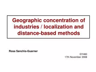
Geographic concentration of industries / localization and distance-based methods. Rosa Sanchis-Guarner GY460 17th November 2008. This seminar. In this seminar we study measures of manufacturing concentration based on 2 papers:

E N D
Geographic concentration of industries / localization and distance-based methods Rosa Sanchis-Guarner GY460 17th November 2008
This seminar • In this seminar we study measures of manufacturing concentration based on 2 papers: • “Evaluating the geographic concentration if industries using distance-based methods”, Eric Marcon and Florence Puech, JEG, 2003. • “Testing for localization using micro-geographic data”, Gilles Duranton and Henry Overman, REG, 2005.
1st paper “Evaluating the geographic concentration if industries using distance-based methods” Eric Marcon and Florence Puech, JEG, 2003
Marcon and Puech, JEG, 2003 (1) • Economic activity is not homogeneously distributed in the space: geographic agglomeration (numerous evidence) • Traditionally concentration indices are used: • Herfindahl, Gini or Ellison-Glaeser • The problem of these indices is that they evaluate the concentration at a single geographical level • an arbitrary geographical level of clusters is chosen we compute the indices for the different levels
Marcon and Puech, JEG, 2003 (2) • This is limited: the authors use distance-based methods to assess the concentration or dispersion of firms: • They can describe spatial distribution at different geographical levels simultaneously • They overcome the circumvent scale problem and the MAUP problem • At different scales we can find different results
Marcon and Puech, JEG, 2003 (3) Intuition: • For each firm we count the number of its neighbours (other firms) within a given distance • We calculate the average number of neighbours for every firm at each distance • The benchmark is complete spatial randomness (CSR): firms locate independently and with the same probability (density) everywhere • If location is not random and firms locate close to other firms because it is attractive, we can expect to find more neighbours than if the location is random • The contrary for dispersion (less neighbours)
Marcon and Puech, JEG, 2003 (4) • To determine if the distribution of firms is different from the CRS we use a mathematical function called L (a modification of Ripley’s K function). • We can have 4 types of distribution: • Homogeneous: constant density • Completely random or independent • Concentration or agglomeration • Dispersion
Marcon and Puech, JEG, 2003 (5) • Ripley’s K function describes the spatial distribution of a set of points • λ is the average density of points (constant) • K(r) is the average number of neighbours divided by λ • For a random distribution, the expected number of points in a circle of radius r is λπr2, so for CRS K(r)=πr2 (benchmark) • The L(r) function is a normalisation of the K function in order to obtain a benchmark of zero • L(r) > 0 the distribution is geographically concentrated • L(r) = 0 the distribution is geographically independent (L is flat) • L(r) < 0 the distribution is geographically dispersed
Marcon and Puech, JEG, 2003 (6) Procedure: • They pick an area of study (rectangular area) • They calculate K and L for a wide range of radius: count the firm’s average number of neighbours within a circle of given radius • The correct for the “edge effect” (factor of the circle's area divided by the intersection area) • They compare the actual distribution of firms differs significantly to the null hypothesis of random distribution • They generate confidence intervals by generating by simulation (Monte Carlo) a big number of independent random distributions with the same number of points and density than the sample of firms
The edge problem illustration radius radius
Marcon and Puech, JEG, 2003 (7) • They use French data on firms (geographic database) on an industrial area around Paris and 14 sectors • Lmin and Lmax limit the interval at which the null hypothesis of random distribution is valid • The associated L curve show significant concentration for all distances to 0 to 25 kms (for all sectors and for total manuf)
Marcon and Puech, JEG, 2003 (8) • Compared to homogeneous distribution: all sectors and all manufacturing are concentrated at different scales. • Then they assess if some sector (particular set of firms) is more concentrated than the industry. • The benchmark is now heterogeneous: we compare the concentration of a sector relative to the average industrial density
Marcon and Puech, JEG, 2003 (9) • In this paper the advantage is that they measure concentration by analysing simultaneously the spatial distribution of firms at different geographical scales • Preserve the continuous setting of the data • Their measure complements the existing measures (indices) • It does not take into account the individual characteristics of firms • Is very computer intensive
2nd paper “Testing for localization using micro-geographic data” Gilles Duranton and Henry Overman, REG, 2005
Duranton and Overman, RES, 2005 (1) • They use distance-based methods to study the location patterns of industries and particularly their tendency to cluster relative to overall manufacturing • Their approach assess the departure from randomness (no location) • The apply it to the UK manufacturing • Their findings (for 4-digit industries): • 52% are localized at a 5% confidence level • Localization takes place mostly at small scales below 50 kms • The degree of localization is very skewed • Industries follow sectoral patterns: smaller and bigger establishments follow different patterns in different industries
Duranton and Overman, RES, 2005 (2) • Localization: tendency of an industry to agglomerate/concentrate over and above the overall economic activity • At which scale this localization occurs? • Normally indices are used to measure localization at different geographical scales • Are small or big establishments the ones which drive concentration?
Duranton and Overman, RES, 2005 (3) Desirable requirements of a localization measure: • Comparable across industries • Control for the general tendency of manufacturing to agglomerate (in some places there is more employment than in others) • Control for industrial concentration (there are factors that make plants cluster in their location) • Gini indices satisfy 1 + 2 • Ellison and Glaeser satisfies 1 + 2 + 3 • Problem with these indices is that they transform dots on a map into units in boxes (waste of information)
Duranton and Overman, RES, 2005 (4) Desirable requirements of a localization measure: • Unbiased with respect to scale and aggregation level (so we do not aggregate the points and we overcome the MAUP problem) • Gives and indicator of statistical significance • Their measure satisfies 1 + 2 + 3 + 4 + 5 • They will use spatial point patterns techniques: • They calculate the distribution of distances between pairs of establishments in an industry • They compare this distribution to with that of a hypothetical industry with the same number of establishments which are randomly distributed conditional of the distribution of aggregate manufacturing
Data: 1996 Annual Respondent Database ARD Information about all the UK establishments They have the postcode of the location (block) They geo-reference the data After solving some problems they have 176,106 locations Each dot represents a production establishment Duranton and Overman, RES, 2005 (5)
Duranton and Overman, RES, 2005 (6) Methodology: • They select the relevant establishments • They compute the density of bilateral distances between all pair of establishments in an industry • They compute the counterfactuals • Same number of establishments • Randomly allocated across the existing sites • They construct the local confidence intervals and the global confidence bands at 5% level: we can compare the actual distribution to the counterfactuals to assess the significance of departures from randomness
Duranton and Overman, RES, 2005 (7) • Step 1: consider a size threshold and only retain establishments with employment above that threshold • Step 2: Kernel estimations of K-densities • For any industry A they calculate the Euclidean distance between any pair of establishments (actual location) • To control for the noise they kernel-smooth when estimating the distribution of bilateral distances • The grid points in the x-axis are 0-180 kms distances • They control for dependence between the bilateral distances => they need to use Monte Carlo simulations to test for departures from randomness
Duranton and Overman, RES, 2005 (8) • Step 3: construct relevant counterfactuals: • The number of firms in each industry and the size distribution is taken as given • To control for the overall tendency of manufacturing to agglomerate they consider the set of existing sites currently use by a manufacturing establishment as the set of all possible locations for any plant • They construct the counterfactuals by first drawing locations from the overall population of sites and then calculating the bilateral distances. • They run 1000 simulations for each industry and calculate the smoothed density for each simulation
Duranton and Overman, RES, 2005 (9) • Step 4: construct the confidence intervals • They draw a sample from the distribution of all manufacturing sites and re-compute the density (step 3) • They restrict the distance grid points to 0-180 kms. • Local: they repeat step 3 1000 times for each distance grid point . The upper and lower bounds to 95% of this density estimates at that distance grid point gives the local confidence interval. The shape of these intervals reflects the distribution of overall manufacturing • Global: they find out which local upper and lower bounds would include 95% of the estimates at every grid point and this are the global confidence intervals. The statement is valid for the overall location pattern of the industry.
Duranton and Overman, RES, 2005 (10) Interpretation: • Local (dotted lines): localization (dispersion) is detected when the K-density of one particular industry lies above (below) its local upper (lower) confidence interval • In the graph: • industry D exhibits localization for every km in [0-60] • Industry C exhibit dispersion in the same range • Global (dashed lines): global localization is detected when the K-density of one particular industry lies above its upper confidence interval. Global dispersion when the K-density lies below the lower confidence band and never lies above the upper confidence band • In the graph: • industry D exhibits global localization • Industry C exhibits global dispersion • Industry B exhibits neither global localization nor dispersion • Industry A exhibits global localization and no dispersion
Duranton and Overman, RES, 2005 (12) • Basic results for the UK firms • 52% of industries are localized, 24% are dispersed and 24% do not deviate from randomness • Localization is not as widespread as found in other studies • Localization takes place at fairly small scales • Deviations from randomness are very skewed across industries • Industries that belong to the same branch tend to have similar localization patterns • Other things they do • Study the effect of the size of the establishment • After censoring for small only 43% show localization • Weight for employment • Compare with EG index • Do it for 3-digits and 5-disgits classification
Duranton and Overman, RES, 2005 (13) Main findings: • 51% of four-digit industries exhibit localisation at a 5% confidence level and 26% of them show dispersion at the same confidence level. • Localisation in four-digit industries takes place mostly between 0 and 50 kilometres. • The extent of localisation and dispersion are very skewed across industries. • Four- and five-digit industries follow broad sector and branch patterns with respect to localisation. • In some industrial branches, localisation at the industry level is driven by larger establishments, whereas in others it is smaller establishments which have a tendency to cluster. • • Localisation and dispersion are as frequent in three-digit sectors as in four-digit industries for distances below 80 kilometres. Three-digit sectors also show a lot of localisation at the regional scale (80 − 140 kilometres) due, at least in part, to the tendency of four-digit industries to co-localise at this spatial scale
Compare both papers • Marcon and Puech compute the number of establishments within a given radios • Duranton and Overman find K as the average number of points located at a distance r from each firm