Singular Perturbation with Variable Fast Time Scales
250 likes | 468 Views
Singular Perturbation with Variable Fast Time Scales. Harvey Lam http://www.princeton.edu/~lam Princeton University September, 2007. Why do reduced models?. To reduce the number of unknowns, To reduce stiffness, To gain insights on the system under investigation. --------

Singular Perturbation with Variable Fast Time Scales
E N D
Presentation Transcript
Singular Perturbation with Variable Fast Time Scales Harvey Lam http://www.princeton.edu/~lam Princeton University September, 2007
Why do reduced models? • To reduce the number of unknowns, • To reduce stiffness, • To gain insights on the system under investigation. -------- Finding a “slow manifold” is not enough.
Analytical asymptotics needs a dimensionless epsilon: <<1 • Generic problem statement (t=O(1)): • What happens when g(y;) is singular in the small limit? (note: w(y) and yo has no singular dependence) • When g(y;) is uniformly singular in the small limit, it is a classical singular perturbation problem. No problem.
Real world problems often have no uniformly small epsilons • Real world problems are usually nonlinear and dimensional. • Most parameters in real world problems are dimensional. • Many interesting real world problems are intractable by pen-and-pencil analysis. • All the Rome ODE benchmark problems have non-uniformly small epsilons.
What do most people do?(for a N variables problem) • Somehow figure out that M of the original N variables are fast. Denote them by r. • The rest of the variables are denoted by s. • Numerically compute for: and call this algebraic relation the Slow Manifold (usefulfor certain initial conditions).
Some details (r is fast, s is slow) • Suppose we arrange the variables so that: • Then the original ODEs are:
How useful is any numerical Slow Manifold r=S(s)? • The original ODEs are: Can we do the following?
Answer: sometimes yes, sometimes no. • Even when epsilon is uniformly small. • It is yes when the chosen r fast variables accept the QSSA---quasi-steady-state-approximation. • It is no when the r fast variables needs the PE---partial equilibrium approximation. • For messy large real world problems, we usually don’t know which is which.
What is “all you need”? • The leading-order Slow Manifold Projector:where am and bm are (column and row) CSP-refined fast basis vectors. They are independent of w(y). • If the CSP bm refinement “converges”, there is a slow manifold right here.
What the CSP-refined basis vectors tell you…. • Here are the projectors: The Slow Manifold after K cycles of 2-step CSP refinement is:
The Reduced Model • After the fast transients die (using Kth-CSP-refined basis vectors): One may remove any M differential equations here and replace them by the M algebraic equations of state in the previous slide. Number of variables is reduced!
The two-step CSP refinement • Step one refines the bm vectors. This provides the slow manifold. • Step two refines the am vectors. This removes stiffness from reduced model. • If the refinement “iterations” for bm does not seem to converge, there is no slow manifold here.
The Williams Problem • CSP form of the system (no approximation)
x is non-uniformly small when is small. (y is QSSA)
The Lindemann Problem CSP form of the problem (exact):
Lindemann is a PE problem! • Leading approximation to slow manifold: is completely correct… but completely useless in the original ODEs---even if is uniformly small.
The Semenov ODE Problem Originals: Introduce a new variable:
More on Semenov ODEs Where plays the role of epsilon:
Coming out of a slow manifold • It is possible for (x,y) to be small for a while, then become a non-small number later. • Solutions with diverse initial conditions would become a tight bunch when they enter into the slow manifold. • When these bunched solutions come out of the slow manifold, they may still look bunched. But appearance of bunching is not sufficient to conclude that there is a slow manifold.
The Semenov PDE Problem • Original PDEs: When diffusion is absent(or if Le=1), T+c is independent of details of the chemistry term. CSP form:
On the non-chemistry term • How does the magnitude of the diffusion term depend on the magnitude of ? • Answer: if diffusion needs to compete (such as near a boundary), it can and will match whatever the chemistry term has to offer! • Whenever this happens, there is no slow manifold (number of unknowns cannot be reduced).
The Davis Skodje Problem • Original ODEs: This ODE follows (without approximation): which is valid even for arbitrary (y1,y2)!
Large and small Slow manifold: (large limit) Conservation Law: (small limit)
Slow manifold versus Conservation Laws • Consider: We get a slow manifold when f1 decays to become small: If fN is always small, AND if bN is the gradient of a scalar, then we get an Approximate Conservation Law for that scalar (e.g. an Hamiltonian and …).
Concluding Remarks • In general, finding a slow manifold is not enough. • A slow manifold should be useful for problems other than the one you found it from. (i.e. good for differentw(y)’s---such as “missing” reactions, any slow perturbations, diffusions, control forces …) • Reduced models should be able to use single precision numerical slow manifolds. • Reduced models should tell you some interesting and insightful things about the system. http:www.princeton.edu/~lam