Time-Dependent Perturbation Theory
Time-Dependent Perturbation Theory. David K. Ferry and Dragica Vasileska Arizona State University Tempe, AZ 85287-5706. 2. 3. 4.

Time-Dependent Perturbation Theory
E N D
Presentation Transcript
Time-Dependent Perturbation Theory David K. Ferry and Dragica Vasileska Arizona State University Tempe, AZ 85287-5706
2 3 4 Objective:To calculate the transition probability from a state |n> to a state |m>.These occur under the influence of a perturbation ,which slightly displaces the system from equilibrium and causes the transition. The perturbation is usually time dependent. To calculate the change in the eigen state Ψ(r ,t) due to the perturbation, V(r ,t), we solve the TDSE. 1 where H0(r) is the operator for the total energy of the unperturbed system and V(r,t) is the perturbing potential. We first consider the unperturbed system The stationary part of the wave function is assumed to satisfy the eigen value equation The solution is then of the form,
5 6 7 8 9 The wave functions form a complete and orthonormal set and so the total wave function can be expressed as a linear combination of the individual eigen functions for each state. Inserting this into the TDSE 1( for the perturbed system), and using equation 3, we get on simplification, We now use the property that two non identical states are orthogonal to each other, by pre multiplying the above equation with and integrating over all space to get:
10 11 Let us assume that we have a harmonic potential. Then and, Substituting this into equation 9, we get, What we have obtained is a complete set of equations for the expansion coefficients am(t) and their time dependence. Matrix methods can be used to solve this problem but it is generally a computationally taxing task. The approach that we adopt is as follows. We assume that initially the system was in a state k before the perturbation is turned on : From the above expression, we have To understand the meaning of these coefficients, consider the normalization of It can also be shown that,
12 13 14 The next task is to calculate the amplitude am(t), from the coupled set of differential equations.If V(r,t) is small perturbation, we can make an approximation that even at t>0 we have, In this case we only have to solve the following equation Integrating this equation from 0 to t, we get 1 0 15 The following can also be shown
15 To summarize, in the limit t->∞, the probability Wmk(t) is The above limit can only be used in the case when one scattering event is finished before the other starts i.e., when the scattering is infrequent . Smk is called transition rate i.e., the probability for the transition in a time of interval t The formula in equation 15 was named by Fermi (as with some measure of importance) “The Golden Rule”. • Summary of approximations made in deriving Fermi’s Golden Rule • Weak perturbation which gives no depletion of the initial state ak(t)=1 for all times • The limit t->∞, can only be used when we are in a weak scattering regime. It led to Energy conservation in the scattering process which is not necessarily satisfied under heavy scattering. • Summary of Notation
Example that illustrates the application of Fermi’s Golden rule Consider a potential barrier of the form : We can view this as a scattering potential. Use Fermi’s Golden rule to calculate the reflection probability and compare it with the exact result of Solution We calculate the matrix element for the scattering event as follows. Evaluating this straight forward integral, The total probability of scattering out of state k is From energy conservation we have |k’|=|k|, but we consider only k’=-k for reflection. Also using the dispersion relation, we convert the integration into Energy domain and the result is Now T in the expression is the time it takes for electrons to cross the length Lz. Therefore If we consider very weak scattering then V0<<E and it is very simple to show that RB(E) reduces to the expression from Fermi’s Golden Rule Fermi’s Golden Rule result
Application 2: Elastic scattering of Electrons Consider the coulomb interaction between a charge center Ze and the electron as a perturbation. The perturbing potential is given by . It should be noted that Coulomb interaction is first order time independent, which means that only the w=0 term will be non zero Before we proceed with the solution, we need to introduce the concept of SCATTERING CROSS SECTION The probability of scattering out of state k is given by Evaluating this, by using the parabolic dispersion relation and reducing the integral to energy domain, we get Physical explanation of scattering cross section • The scatterer can be viewed as a solid obstacle with cross sectional area σs which scatters a fraction of the incident electrons equal to σs/A. • Usually we have electrons moving through a medium of certain density (Ni) of scattering centers and we need to find the probability that an electron is scattered in time t . • Since each scatterer scatters σs/A fraction of electrons, the total number of scatterers encountered in that time t is, NiAVt. • Therefore, Ps(t)=σs/A* NiAVt=t/τ, where τ is the mean time between scattering events Again, T in the expression is the time it takes for electrons to cross the length Lz. Therefore, To get the total scattering cross section, we need to integrate over entire solid angle
Therefore to evaluate T, we need to find the total scattering cross section. where, The matrix element is calculated from The volume of the box to which we normalize all wave functions is completely arbitrary and unphysical and will never appear in the final result for some measurable quantity. We now define β=k’-k, as being the momentum transfer in the scattering process. Since we have freedom in choosing the coordinate system, we can chose β to be aligned with the z-axis, β.r= βr cosθ If then scattering is isotropic as and if then Scattering is anisotropic and peaked around θ=0; High energy electrons are hardly deflected Low energy electrons
To get the total cross section, we need to integrate over the entire solid angle to get Brooks Herring result When Ld ->∞ (depletion region of a semiconductor), σs and are large. It is important to note that once Ld gets comparable to the inter impurity spacing, (~ Ni-1/3), the coulomb potential of nearby impurities overlap. It is then necessary to modify the Brooks Herring theory. More appropriate in those cases is the Conwell - Weisskopf theory, which is not discussed here.