Discrete-Time Convolution
Discrete-Time Convolution. Discrete-time Convolution. Output y [ n ] for input x [ n ] Any signal can be decomposed into sum of discrete impulses Apply linearity properties of homogeneity then additivity Apply shift-invariance Apply change of variables. y [ n ]. x [ n ]. System.

Discrete-Time Convolution
E N D
Presentation Transcript
Discrete-time Convolution • Output y[n] for inputx[n] • Any signal can be decomposedinto sum of discrete impulses • Apply linearity properties ofhomogeneity then additivity • Apply shift-invariance • Apply change of variables
y[n] x[n] System h[n] Averaging filter impulse response n 0 1 2 3 Discrete-time Convolution • Filtering viewpoint Hold impulse response h[n] in place and change variables Flip and slide input signal x[n] about impulse response • Example of finite impulse response (FIR) filter Impulse response has finite extent (non-zero duration) y[n] = h[0] x[n] + h[1] x[n-1] = ( x[n] + x[n-1] ) / 2
Convolution in Both Domains • Continuous-time convolution of x(t) and h(t) For each value of t, we compute a different (possibly) infinite integral. Discrete-time definition is the continuous-time definition with integral replaced by summation • Linear time-invariant (LTI) system Output signal in time domain is convolution of impulse response and input signal Impulse response uniquely characterizes the LTI system
Convolution Demos • Johns Hopkins University Demonstrations http://www.jhu.edu/~signals Convolution applet to animate convolution of simple signals and hand-sketched signals Convolve two rectangular pulses of same width gives a triangle (see handout E) • Some conclusions from the animations Convolution of two causal signals gives a causal result Non-zero duration (called extent) of convolution is sum of extents of two signals being convolved minus one
Fundamental Theorem • The Fundamental Theorem of Linear Systems If one inputs a complex sinusoid into an LTI system, then the output will be a complex sinusoid of the same frequency that has been scaled by the frequency response of the LTI system at that frequency Scaling may attenuate the signal and shift it in phase Example in continuous time: see handout G Example in discrete time. Let x[n] = e j Wn,H(W) is the discrete-time Fourier transform of h[n] and is also called the frequency response
Frequency Response • For continuous-time LTI system • For discrete-time LTI system • Note: Identity for cosine input assumes a real-valued impulse response
passband Example Frequency Response • System response to complex exponential e j W n for all possible frequencies Win rad/sample • Passes low frequencies, a.k.a. lowpass filter |H(W)| H(W) stopband stopband W W -Ws -Wp Wp Ws Phase Response Magnitude Response
Continuous Discrete f(t) y(t) f[n] y[n] Differentiator/Difference Operation We can remove scaling by 1/Ts without changing lowpass response
First-Order FIR Filters x[n] y[n] = ½ x[n] + ½ x[n-1] y[n] = ½ x[n] ½ x[n-1] n n Signal with a spike Output of averaging filter signal = [ 1 1 1 1 1 10 1 1 1 1 1 ]; figure(1); stem(signal); n Output of difference filter averagingFilter = [ 0.5 0.5 ]; average = conv(averagingFilter, signal); figure(2); stem(average); differenceFilter = [ 0.5 -0.5 ]; difference = conv(differenceFilter, signal); figure(3); stem(difference);
h[n] First-order difference impulse response n Mandrill Demo (DSP First) • First-order difference FIR filter Highpass filter (sharpensinput signal) Impulse response is {1, -1} • Five-tap discrete-time (scaled) averaging FIR filter with input x[n] and output y[n] Lowpass filter (smooth/blur input signal) Impulse response is {1, 1, 1, 1, 1}
Mandrill Demo (DSP First) • DSP First, Ch. 6, Freq. Response of FIR Filters, http://www.ece.gatech.edu/research/DSP/DSPFirstCD/ • From lowpass filter to highpass filter original image blurred image sharpened/blurred image • From highpass to lowpass filter original image sharpened image blurred/sharpened image • Frequencies that are zeroed out can never be recovered (e.g. DC is zeroed out by highpass filter) • Order of two LTI systems in cascade can be switched under the assumption that computations are performed in exact precision
Mandrill Demo (DSP First) • Input image is 256 x 256 matrix Each pixel represented by eight-bit number in [0, 255] 0 is black and 255 is white for monitor display • Each filter applied along row then column Averaging filter adds five numbers to create output pixel Difference filter subtracts two numbers to create output pixel • Full output precision is 16 bits per pixel Demonstration uses double-precision floating-point data and arithmetic (53 bits of mantissa + sign; 11 bits for exponent) No output precision was harmed in making of this demo
Linear Time-Invariant System • Any linear time-invariant system (LTI) system, continuous-time or discrete-time, can be uniquely characterized by its Impulse response: response of system to an impulse Frequency response: response of system to a two-sided complex exponential input signal for all possible frequencies Transfer function: Laplace transform (or z-transform) of impulse response • Given one of the three, we can find other two provided that they exist May or may not exist May or may not exist