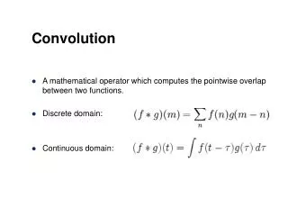
Convolution
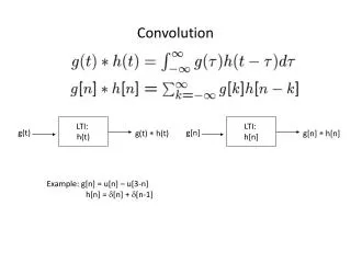
Convolution. LTI: h(t). LTI: h[n]. g(t). g[n]. g(t) h(t). g[n] h[n]. Example: g[n] = u[n] – u[3-n] h[n] = [n] + [n-1]. Convolution methods:. Method 1: “running sum” Plot x and h vs. m Flip h over vertical axis to get h[-m] Shift h[-m] to obtain h[n-m]

Convolution
E N D
Presentation Transcript
Convolution LTI: h(t) LTI: h[n] g(t) g[n] g(t) h(t) g[n] h[n] Example: g[n] = u[n] – u[3-n] h[n] = [n] + [n-1]
Convolution methods: • Method 1: “running sum” • Plot x and h vs. m • Flip h over vertical axis to get h[-m] • Shift h[-m] to obtain h[n-m] • Multiply to obtain x[m]h[n-m] • Sum on m, m x[m] h[n-m] • Increment n and repeat steps 3~6
Convolution methods: • Method 2: Superposition method • We know [n] h[n] and the system is LTI. • Therefore, a0[n-n0] a0h[n-n0] • a0[n-n0] + a1[n-n1] + … a0h[n-n0] + a1h[n-n1] … • Since the input can be expressed as a sum of shifted unit samples: x[n] = … x[-2][n+2] + x[-1][n+1] + x[0][n] + x[1][n-1] + … • The out is then a sum of shifted unit sample responses: x[n0][n-n0] + x[n1][n-n1] + … x[n0]h[n-n0] + x[n1]h[n-n1] … 1k=-1x[k]h[n-k] (The Convolution Sum!)