Download
1 / 28
300 likes | 545 Views
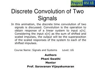
Discrete Convolution of Two Signals.

E N D
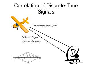
Discrete Convolution of Two Signals In this animation, the discrete time convolution of two signals is discussed. Convolution is the operation to obtain response of a linear system to input x[n]. Considering the input x[n] as the sum of shifted and scaled impulses, the output will be the superposition of the scaled responses of the system to each of the shifted impulses. Course Name: Signals and Systems Level: UG Authors Phani Swathi Mentor Prof. Saravanan Vijayakumaran
Learning Objectives After interacting with this Learning Object, the learner will be able to: • Explain the convolution of two discrete time signals
Definitions of the components/Keywords: 1 • Convolution of two signals: • The x[n] and h[n] are the two discrete signals to be convolved. • The convolution of two signals is denoted by • which means • where k is a dummy variable. 2 3 4 5
Master Layout (Part 1) This animation consists of 2 parts: Part 1 – First method of convolution – Method 1 Part 2 – Alternate method of convolution – Method 2 1 Lines and dots have to appear at the same time. This is applicable to all figures Signals taken to convolve Shifted version of h[n] Scaled version of h[n] 2 3 4 5
Step 1: 1 2 3 4 5
Step 2: Overall calculation of y[n] 1 X[1]h[n-1] 3 2 1 2 0 1 2 3 n X[2]h[n-2] h[n-2] 6 4 2 3 2 1 3 0 1 2 3 4 n 0 1 2 3 4 n h[n-3] 3 2 1 X[3]h[n-3] 3 2 1 4 0 1 2 3 4 5 n 0 1 2 3 4 5 n 5
Step 3: 1 X[1]h[n-1] x[1]h[n-1] 3 2 1 2 0 1 2 3 n 3 4 5
Step 4: Step 1 1 X[2]h[n-2] 6 5 4 3 2 1 h[n-2] X[2] h[n-2] 3 2 1 2 2 3 0 1 2 3 4 n 0 1 2 3 4 n 4 4 5 5
Step 5: 1 X[3]h[n-3] h[n-3] x[3]h[n-3] 3 2 1 3 2 1 2 3 0 1 2 3 4 5 n 0 1 2 3 4 5 n 4 5
Step 6: Y[n] 1 1 8 7 6 5 4 3 2 1 Y[n] 2 2 3 0 1 2 3 4 5 6 7 8 n 4 4 5 5
Electrical Engineering Use STAM template Slide 1 Slide 3 Slide 26 Slide 28 Slide 27 Introduction Definitions Analogy Test your understanding (questionnaire) Lets Sum up (summary) Want to know more… (Further Reading) Interactivity: The correct answer is shown in red Try it yourself Fig. A Fig. B Fig. C Fig. 1 Fig. 2 Demo Activity Fig. A Fig. C Fig. B 11 Instructions/ Working area Credits
Interactivity option 1: Step No 1: 1 y[n] h[n] x[n] 3 2 1 3 2 1 3 2 1 2 0 1 2 3 4 5 0 1 2 3 4 5 3 Fig. 1 Fig. 2 0 1 2 3 4 5 n -1 0 1 2 3 4 5 n Fig.1 Fig.2 4 5
Interactivity option 1: Step No 2: 1 y[n] Y[n] Y[n] 12 10 8 6 4 2 12 10 8 6 4 2 3 2 1 2 0 1 2 3 4 5 0 1 2 3 4 5 3 Fig. 1 Fig. 2 0 1 2 3 4 5 6 n 0 1 2 3 4 5 6 n a) Fig. A b) Fig. B 4 5
Interactivity option 1: Step No 3: 1 y[n] Y[n] 12 10 8 6 4 2 3 2 1 2 0 1 2 3 4 5 0 1 2 3 4 5 3 Fig. 1 Fig. 2 0 1 2 3 4 5 6 n c) Fig. C 4 5
Master Layout (Part 2) 1 This animation consists of 2 parts: Part 1 – First method of Convolution – Method 1 Part 2 – Alternate method of Convolution – Method 2 Signals taken to convolve h[n] X[n] 2 1 2 3 ……. -3 -2 -1 0 1 2 3 ……. 3 Result signal of convolution The dotted lines represent y[n] The thicker line represents only y[4] 4 5
Step 1: 1 X[n] h[n] 2 2 1 2 3 n 3 ….-3 -2 -1 0 1 2 3….. 4 5
Step 2: 1 h[n-k] X[k] 3 2 2 1 2 k=n-2 k=n-1 k= n k 3 -3 -2 -1 0 1 2 3 4 5
Step 3: 1 2 3 4 5
Step 4: 1 X[k] h[4-k] 2 2 3 4 k 3 -3 -2 -1 0 1 2 3 4 5
Step 5: 1 X[k]h[4-k] X[k]h[4-k] 6 4 2 2 2 3 4 3 4 5
Step 6: Y[4] 1 1 12 10 8 6 4 2 Y[4] 2 2 3 0 1 2 3 4 5 6 7 8 9 n 4 4 5 5
Electrical Engineering Use STAM template Slide 1 Slide 3 Slide 26 Slide 28 Slide 27 Introduction Definitions Analogy Test your understanding (questionnaire) Lets Sum up (summary) Want to know more… (Further Reading) Interactivity: Try it yourself Fig. a Fig. b Fig. c Fig. 3 Fig. 4 Demo Activity Fig. a Fig. b Fig. c 22 Instructions/ Working area Credits
Interactivity option 1: Step No 1: 1 y[n] x[n] h[5-k] 3 2 1 3 2 1 4 3 2 1 2 0 1 2 3 4 5 0 1 2 3 4 5 3 Fig. 1 Fig. 2 0 1 2 3 4 5 6 n 0 1 2 3 4 5 6 n Fig.3 Fig.4 4 5
Interactivity option 1: Step No 2: 1 y[n] 4 3 2 1 3 2 1 3 2 1 Y[5] Y[5] 2 0 1 2 3 4 5 0 1 2 3 4 5 3 Fig. 1 Fig. 2 0 1 2 3 4 5 6 n 0 1 2 3 4 5 6 n a) Fig. a b) Fig. b 4 5
Interactivity option 1: Step No 3: 1 y[n] Y[5] 4 3 2 1 3 2 1 2 0 1 2 3 4 5 0 1 2 3 4 5 3 Fig. 1 Fig. 2 0 1 2 3 4 5 6 n c) Fig. c 4 5
Questionnaire 3 2 1 1 3 2 1 1. Find the value of y[6] Answers: a) b) 2.The Convolution sum is given as ___________ Answers: The correct answers are given in red. h[n] x[n] 2 0 1 2 3 4 5 6 0 1 2 3 4 5 6 10 8 6 4 2 8 6 4 2 3 4 0 1 2 3 4 5 6 0 1 2 3 4 5 6 5
Linksfor further reading Reference websites: Books: Signals & Systems – Alan V. Oppenheim, Alan S. Willsky, S. Hamid Nawab, PHI learning, Second edition. Research papers:
Summary • In discrete time, the representation of signals is taken to be the weighted sums of shifted unit impulses. • This representation is important, as it allows to compute the response of an LTI(Linear Time Invariant) system to an arbitrary input in terms of the system’s response to a unit impulse. • The convolution sum of two discrete signals is represented as where • The convolution sum provides a concise, mathematical way to express the output of an LTI system based on an arbitrary discrete-time input signal and the system‘s response.