Download
1 / 36
360 likes | 588 Views
Solar and Interplanetary Modeling. Janet Luhmann and the Solar CISM Modeling Team. Coupled Modeling Scheme. Solar Corona SAIC. Solar Wind ENLIL. Magnetosphere LFM. Ionosphere T*GCM. SEP. MI Coupling. Active Regions. Ring Current. Geocorona and Exosphere. Radiation Belts. Inner

E N D
Solar and Interplanetary Modeling Janet Luhmann and the Solar CISM Modeling Team
Coupled Modeling Scheme Solar Corona SAIC Solar Wind ENLIL Magnetosphere LFM Ionosphere T*GCM SEP MI Coupling Active Regions Ring Current Geocorona and Exosphere Radiation Belts Inner Magnetosphere Solar CISM Plasmasphere
Solar CISM Organizational Activities Since STC Selection • Participated in BU Kickoff Meeting (Sept. ‘02) • Met with collaborators at ‘02 SPD and SHINE Meetings • Posted SolarCISM website (http://sprg.ssl.berkeley.edu/cism) • Collaborated on CISM-related SF Exploratorium EPO proposal to NASA IDEAS Program • Held first annual SSL SolarCISM meeting in Dec. ‘02 (26 participants from 14 institutions) • Advertised two UCB CISM positions (NRL liaison and UCB Senior Fellow for SEP), also filled HAO liaison position • Interacted with KT group on CISM Empirical Model contribution for corona/solar wind (Arge) • Identified potential Access Grid rooms at UCB, SAIC, Stanford now working with BU to purchase and install equipment • Participated in bimonthly executive telecons • Multi-institution working subgroups met at HAO/U of Colo., UCB, and SAIC
Solar CISM WebsiteNow Available • http://sprg.ssl.berkeley.edu/cism
SAIC and CIRES/NOAA SEC Coronal and Heliospheric Modeling For CISM: Pre-STC and 1st Year CISM Results • Performed propagation of 2D CME in the coupled model, studied results. • Performed large-angle 3D CME in the coupled model. • Performed 3D simulation of emerging Active Region. • Developing new MPI version of the coronal code which is currently in testing. • Introduced rotation into the 2D CME calculation: spiral magnetic field modifies shock characteristics. • Investigated in situ properties of simulated CMEs.
Coronal/Heliospheric Modeling For CISM (Continued) • Developing new MPI version of the coronal code which is currently in testing. • Introduced rotation into the 2D CME calculation: spiral magnetic field modifies shock characteristics. • Investigated in situ properties of simulated CMEs. • Studied the extension of the Wang-Sheeley approach using the NOAA/SEC heliospheric MHD model. • Investigated STEREO views of a simulated CME. • Publications: 1) Odstrcil et al., J. Geophys. Res. 107, 10.1029/2002JA009334, 2002 2) Riley et al., Astrophys. J. 578, 972, 2002 3) Linker et al., Phys. Plasmas, to appear, 2003
Current SAIC + U. Colorado CISM EffortTwo dimensional flux rope eruption simulation undergoing improvements (e.g. in coronal/solar wind model coupling and spatial resolution)
Expanding Magnetic Flux Rope - Initial 3D Version Developed Shock Model Interface Ejected Plasma Magnetic Leg Compressed Plasma
Evidence of Post-Eruption Reconnection Jet - samples of visualizations and diagnostics
Conditions for Energetic Particles Magnetic Field Lines Shock Front Surface theta = 60 deg theta = 70 deg theta = 80 deg theta = 90 deg • Magnetic field lines, as observed at given locations can be: • part of the magnetic flux rope; • connected to the solar surface; or • disconnected from the solar surface.
Multi-Perspective Imaging - sample of application to heliospheric imaging observations from SMEI and STEREO
UCB + SAIC Emerging active region magnetic fields effects on the coronal field configuration Steps to provide constructed magnetic field maps to SAIC to be the boundary condition for their MHD models: • Perform a local ANMHD simulation of an emerging fluxrope. • Use the radial component of the fluxrope as it emerges up into the photosphere to be the active region field. • Make a global background field, i.e., a dipole field. • Insert the series of simulated active region field into the background field. • SAIC uses the series of synthetic synoptic maps as boundary condition and starts with a potential field to perform their global MHD model to generate coronal field lines, coronal hole areas and coronal streamer belt images.
Current UCB + SAIC CISM EffortInitiation of Coronal Eruptions UCB simulation of emergence of an active region from below the photosphere into the corona –provides sample boundary conditions for the SAIC corona model.
Current UCB + SAIC Effort(continued) a) Transverse magnetic field vectors b) Transverse velocity vectors and radial magnetic field contours The simulated emerging active region model coupling tells us how to better use observations to drive the coronal model.
Left: ANMHD flux rope as it emerges up to the photosphere. Field lines are overplotted on the gray scale active region images. Right: constructed global magnetic field maps using a dipole background and the radial component of the emerging flux rope simulation.
SAIC’s global MHD model results using the constructed maps as the inner boundary condition. The evolving photospheric field maps are here shown in a blue-white-red color scheme. The green lines are initially closed field lines, and black lines are initially open. SAIC’s global MHD model results. The green lines are initially closed field lines, and black lines are initially open. The dark gray areas are coronal holes.
A different perspective of the global MHD field lines with the active region located at the right side. As the active region emerges, the field lines and streamer belt are distorted. Simulated coronal images using the plasma density of the MHD model to calculate polarization brightness (pB). The streamer belt on the right is distorted and separates into two streamers. The transient behavior is under investigation.
HAO + U of Colorado + NOAA/SEC + UCB + Lockheed CISM Effort HAO Synoptic map project (de Toma, Arge, Gibson, & Mayer) Global coronal magnetic field-solar wind relationships (Gibson & Arge) NOAA/SEC Wang-Sheeley-Arge (WSA) empirical coronal/solar wind model (Arge, Pizzo, & Mayer) WSA coronal and Odstrcil MHD solar wind model coupling (Odstrcil, Arge, & Pizzo) CU/LASP Incorporation of the WSA model into the CISM Sun-to-Earth Empirical Model (CSEM) (Baker, Weigel, Arge, & Mayer) UC Berkeley Solar event studies (Luhmann, Arge, & Li) Lockheed Incorporation of Schrijver-Derosa photospheric field evolution model into WSA. (Arge, Schrijver, & DeRosa)
HAO + U of Colorado + StanfordSynoptic Map Projects At HAO: • Routine construction of solar/coronal synoptic maps • He 10830 Å • H (HAO) • White light • Photospheric field (NOAA/SEC) • IDL software package will be made available to solar community.
HAO + U of Colorado + StanfordSynoptic Map Projects At Stanford: Magnetic field from WSO Magnetic field from MDI mag Event-specific modified maps Intensity from MDI EIT 171Å EIT 254Å EIT 195Å EIT 304Å
Coupled Model: PFSS+SCS Schatten Current Sheet Model (SCS): 2.5 – 21.5 R 21.5 R 2.5 R L1 Near Solar Minimum Near Solar Maximum U of Colorado + NOAA/SEC Empirical Wang-Sheeley-Arge Model provided to CISM KT group 1D Modified Kinematic Solar Wind Model Potential Field Source Surface Model (PFSS): 1.0 – 2.5 R
Level 1 Data Flow Diagram for WSA IDL Fortran 5 3 PERL 2 Assemble latest WSO Daily Updated Synoptic Map Latest Synoptic Map 4 Generate Date File 6 Predict Solar Wind Speed and IMF Polarity at 1 AU 8 Retrieve Last 24 Hours of ACE Velocity & IMF Observations 7 Plot Photospheric Field, Derived Coronal Holes, Source Surface Field, Solar Wind Speed 9 Plot Solar Wind Speed and IMF Polarity Predictions Against Real-Time ACE Observations Magnetograms Convert LOS Photospheric B Field to Radial, Interpolate Grid, & Subtract Monopole 1 Retrieve Latest WSO Magnetograms Interpolated Map Date, Time, File name of Synoptic Maps Potential Field Source Surface Model with Field Line Tracing Date File for Last Three Rotations Output from Previous PFSS Model Runs (Last 3 Rotations) Photospheric Field Derived Coronal Holes Source Surface Field Field Expansion Factor Hourly Ace DATA Solar Wind Speed and IMF Polarity Predictions for Last Three Rotations
U of Colorado + NOAA/SEC WSA Coronal - Odstrcil MHD Solar Wind Model Coupling • PFSS model now generalized to work for different grid resolutions. • A new & improved photospheric field remapping routine written. • Work on improving the interface between the models. • Working to inter-calibrate models better.
Calibration Study – Near Solar Minimum( CR 1954 ) 0.1 AU 1 AU Low inclination of the streamer belt causes difficulties in timing of fast streams
Calibration Study – Near Solar Maximum( CR 1954 ) 0.1 AU 1 AU • Source-Surface models are applicable at solar maximum • Amplitudes need to be balanced
Selected CISM Solar Event: May 12, 1997 CME Photospheric field from SOHO MDI SOHO EIT EUV observations SOHO LASCO C2 and C3 observations
Selected CISM Solar Event: May 12, 1997 CME (continued) • This flare was probably caused by magnetic cancellation • The filament disappeared during the flare but did not appear to erupt Hiraiso/CRL H_alpha SOHO MDI Magnetograms
Selected CISM Solar Event: May 12, 1997 CME (continued) WIND and SAMPEX observations
UCB + SAIC + Stanford Driving MHD codes with sequences of magnetograms • Physically consistent evolution at bottom plane in a simulation: Terms on LHS describe evolution driven by horizontal motion; RHS describes evolution due to flux emergence or submergence • This requires knowledge of vector components of B and v. • How do we determine v self-consistently from a sequence of vector magnetograms (which give only B)? • Price for ignoring the problem: Incorrect coronal magnetic topology
UCB + SAIC + Stanford Driving MHD codes with sequences of magnetograms Vector magnetic field data show no obvious change before and after the flare.
UCB + SAIC + Stanford (continued) Exploring methods for finding the velocity boundary conditions: AR 8038 May 12, 1997 • Stokes Profiles could be used to get vz • Local Correlation Tracking (LCT) can find a velocity field v (But is it correct?) • Vertical component of induction equation provides a constraint equation on v from a sequence of vector magnetograms (but solution is under-constrained) • Kusano et al. used combination of LCT and vertical induction equation to solve for vz • Longcope has developed a solution by adding an additional constraint: minimize the horizonal kinetic energy. Method appears to work in some cases, but not yet thoroughly tested.
UCB + SAIC + Stanford (continued) Stanford force-free models may help set up the initial conditions for MHD simulations Active region field lines Synoptic display of global field lines 1.0-1.4 Rs Non-linear force-free models Potential field models
UCB + SAIC + Stanford (continued) • Non-linear force-free fields contain free energy to be released in the eruptive events, while the potential field doesn’t. Extrapolation of the force-free field incorporates all three components of the magnetic field, and therefore reflects a more realistic structure of the corona. • Description of non-linear force-free field modeling approach • The technique used is the Boundary Element Method (BEM) developed by Yan, et al. ( Yan & Sakurai, 2000); • The technique needs the three components of the magnetic field at the surface as inputs; • To prepare the vector magnetograms for boundary conditions: • compute potential field from the synoptic maps of magnetic field; • obtain the three components of the potential field on the surface; • replace the vector field data where observation of vector magnetic field are unavailable.
Solar Wind Speed Predictions & Observations Solar Wind Speed at Source Surface (2.5Rs) Observations Predictions IMF Polarity Predictions & Observations Derived Coronal Holes and Photospheric Field Polarity U of Colorado and UCB Solar Event: May 12, 1997 Solar Wind and Stream Context Stream source region May 12th CME Stream source region (suggests solar wind stream following the ICME comes from the southern hemisphere)
Solar CISM Modeling Near-Term Issues and Challenges • Improve ambient solar wind MHD simulation to give realistic speeds and stream structure • Collect needed resources for model coupling and driving (e.g. potential or force-free field models and/or synoptic maps as initial states + boundary conditions, vector magnetograms) • Develop solar energetic particle (SEP) modeling capability • Establish NRL connection • Standardize simulation and other data formats and visualization tools • Track progress (e.g. against implementation plan, metrics)