Enhanced Magnetic Field Modeling Technique for Space Weather Analysis
Improve space weather analysis using a refined magnetic field modeling procedure with updated methodologies and statistical models. The process involves finding boundaries, incorporating IMF values, adding model vectors, and conducting spherical harmonic fits. The model enhances accuracy, with notable differences in North and South magnetic fields showcased through various data comparisons. Updates include transitioning from a dipole field to IGRF, changing error weightings, and adjusting SHF procedures. This advanced approach offers precise results with significant developments in magnetic field modeling.

Enhanced Magnetic Field Modeling Technique for Space Weather Analysis
E N D
Presentation Transcript
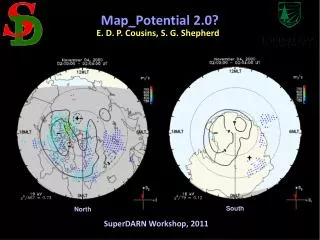
Map_Potential 2.0? E. D. P. Cousins, S. G. Shepherd South North SuperDARN Workshop, 2011
Map_Potential Procedure • Find Heppner Maynard boundary • Get IMF values • Add statistical model vectors • Do spherical harmonic fit (SHF)
Map_Potential Procedure • Find Heppner Maynard boundary • Get IMF values • Add statistical model vectors • Do spherical harmonic fit (SHF)
Map_Potential Procedure • Find Heppner Maynard boundary • Get IMF values • Add statistical model vectors • Do spherical harmonic fit (SHF)
Map_Potential Procedure • Find Heppner Maynard boundary • Get IMF values • Add statistical model vectors • Do spherical harmonic fit (SHF)
Updates • Magnetic Field Model • Dipole → IGRF • Changes model vector calculation and SHF procedure • Statistical model data error weighting • Uniform → Variable • Changes SHF procedure • Statistical Model • RG96 → CS10 [Cousins and Shepherd, JGR, 2010] • Changes model vector calculation
Magnetic Field Model Dipole field IGRF field Difference 50° North -50° South
Magnetic Field Model North December 04, 2000 08:00 – 08:02 UT Dipole IGRF Difference 63 kV χ2/359=1.14 Over 72 hours: Average ΦPC Diff = 2% RMS Diff = 2kV 2%
Magnetic Field Model South December 04, 2000 08:00 – 08:02 UT Dipole IGRF Difference 60 kV χ2/267=2.00 Over 72 hours: Average ΦPC Diff = -4.5% RMS Diff = 1.6 kV -6%
Heppner Maynard Boundary South January 05, 2004 03:20:00 – 03:20:22 UT Original No default HMB latitude • With no data: Original procedure sets HMB = 62° • New procedure uses model lower limit
Model Data Weighting North April 22, 2001 11:00 – 11:10 UT Org. Weighting New Weighting 89 kV χ2/107=1.74 • Model vector errors: • Original: dependent on order of fit and on average of data errors • New: Original value, scaled by number of data vectors in vicinity
Model Data Weighting North April 22, 2001 11:00 – 11:10 UT Org. Weighting New Weighting
Model Data Weighting North April 22, 2001 11:00 – 11:10 UT Org. Weighting New Weighting Difference 89 kV χ2/107=1.74 Average Difference over 24 hours < 1% 4%
Model Data Weighting South May 12, 2001 12:00 – 12:02 UT Org. Weighting New Weighting Difference 71 kV χ2/166=1.74 Average Difference over 24 hours ≈ 1% 3%
Statistical Model RG96 model Fit w/ RG96 North April 01, 2000 18:32 – 18:34 UT Difference 68 kV -34 38 Fit w/ CS10 CS10 model 15% Average Difference over 72 hours ≈ 1% (≈ 3% in summer ≈ -7% in winter)
Statistical Model RG96 model Fit w/ RG96 South March 06, 2000 06:00 – 06:10 UT Difference -43 19 Fit w/ CS10 CS10 model -22% • Average Difference over 72 hours ≈ -12% • (≈-7% in summer • ≈ -9% in winter) 62 kV
Total Difference North April 01, 2000 18:32 – 18:34 UT Original New Difference 87 kV χ2/300=1.95 By = -2.6 nT Bz = -10.7 nT Average Difference over 72 hours ≈ 3% Diff due to new model: 11 kV 15% 21%
Total Difference South March 06, 2000 06:00 – 06:10 UT Original New Difference 61 kV χ2/86=1.41 By = -5.7 nT Bz = -7.1nT Average Difference over 72 hours ≈ -8% Diff due to new model: -17 kV -22% -20%
Total Difference New Difference By, Bz = 0, -6.2 nT • Often little or no difference when data coverage is excellent
Total Difference -2.2 % -2.7 %
Total Difference 2.0 % -4.3 %
Total Difference 5.9 % -3.0 %
Summary • Magnetic Field Model: Dipole → IGRF • Statistical data error weighting: Uniform → Variable • Statistical Model: RG96 → CS10
Summary • Magnetic Field Model: Dipole → IGRF • Statistical data error weighting: Uniform → Variable • Statistical Model: RG96 → CS10 • Small (0 – 10%) average offset between new & old ΦPC • RMS difference between patterns is typically • 2-4 kV in North, 6-8 kV in South (mostly due to new model) • Up to 20 – 30% change in individual patterns’ ΦPC with moderate to low data coverage
Summary • Magnetic Field Model: Dipole → IGRF • Statistical data error weighting: Uniform → Variable • Statistical Model: RG96 → CS10 • Small (0 – 10%) average offset between new & old ΦPC • RMS difference between patterns is typically • 2-4 kV in North, 6-8 kV in South (mostly due to new model) • Up to 20 – 30% change in individual patterns’ ΦPC with moderate to low data coverage • Still needed: get IMF data from OMNI • More robust time shifting

