Really Uncertain Business Cycles
170 likes | 308 Views
Really Uncertain Business Cycles Nick Bloom (Stanford & NBER) Max Floetotto (Stanford) Nir Jaimovich (Stanford). Firm uncertainty appears to be counter-cyclical. Firm-linked uncertainty appears to rise in recessions: Cross-section variation across firms (micro)

Really Uncertain Business Cycles
E N D
Presentation Transcript
Really Uncertain Business Cycles Nick Bloom (Stanford & NBER)Max Floetotto (Stanford)Nir Jaimovich (Stanford)
Firm uncertainty appears to be counter-cyclical • Firm-linked uncertainty appears to rise in recessions: • Cross-section variation across firms (micro) • Time-series variation over months/quarters (macro) • Cross-forecaster disagreement (signal?)
Cross-sectional spread: sales growth Shaded areas are recessions Correlation with GDP growth is -0.404(p-value 0.000) Notes: All firms with at least 25 years of quarterly accounts used (to reduce the impact of compositional changes). Only quarters with at least 500 firms kept to ensure sufficient sample size. Produces a continuous quarterly series from 1967Q2 until 2004Q2. Sales growth spread is defined as the inter-quartile range (IQR) across firms within each quarter, where the IQR is used to minimize the impact of large outliers (mergers, acquisitions, disposals, etc..). Sales growth is defined over a four quarter period to remove the effects of the quarterly accounting cycle, with this centered around the current quarter so that (Sales Growth)t = (Salest+2 - Salest-2)/(0.5хSalest+2 + 0.5хSalest-2). Quarterly recession indicator defined as starting the first quarter after the (NBER defined) business cycle-peak and ending at the (NBER defined) business cycle-trough.GDP growth correlations defined using real quarterly GDP growth.
Cross-sectional spread: firm stock returns Shaded areas are recessions Correlation with GDP growth is -0.423(p-value 0.000) Notes: All firms with at least 25 years of quarterly returns used (to reduce the impact of compositional changes). Only quarters with at least1 1000 firms kept to ensure sufficient sample size. Produces a continuous quarterly series from 1968Q3 until 2006Q1. Stock returns spread calculation using the inter-quartile range (IQR) across firms within each quarter, where the IQR is used to minimize the impact of large outliers (mergers, acquisitions, disposals, etc..). Quarterly recession indicator defined as starting the first quarter after the (NBER defined) business cycle-peak and ending at the (NBER defined) business cycle-trough.GDP growth correlations defined using real quarterly GDP growth.
Time-series volatility: industrial-production growth Shaded areas are recessions Correlation with GDP growth is -0.448(p-value 0.000) Notes: Industrial production standard-deviation (SD) defined as predicted SD from a regression of monthly log industrial production (Final products and non-industrial supplies seasonally adjusted, FRB Statistics) on its own 12 lags, with an ARCH(2) error term. Longer lags in industrial productions or the ARCH error term were not significant (nor was a GARCH MA error term). Quarterly values of SD averaged over the monthly values within the quarter. Recession indicator defined as starting the first month after the (NBER defined) business cycle-peak and ending at the (NBER defined) business cycle-trough. GDP growth correlations defined using real quarterly GDP growth.
Note on estimation of industrial-production volatility(plotted in previous slide) Estimated an AR(12) forecast for log industrial production with an ARCH(2) variance, using monthly data pt = α0 + α1pt-1 + α2pt-2 + …. α12pt-12 + et where et ~ N(0,σt) σ2t = β0 + β1σ2t-1 +β2σ2t + vt where vt ~ N(0,1) σt is the measure of uncertainty plotted in the previous Figure Selected AR(12) and ARCH(2) by testing down from higher order lags and MA series in the AR and GARCH processes
Time-series volatility: stock-market volatility Shaded areas are recessions Correlation with GDP growth is -0.350(p-value 0.000) Notes: Stock market volatility used actual quarterly standard deviation of daily returns until 1987, and average quarterly implied volatility from 1987 onwards (see Bloom, 2007 for details). Quarterly recession indicator defined as starting the first quarter after the (NBER defined) business cycle-peak and ending at the (NBER defined) business cycle-trough. GDP growth correlations defined using real quarterly GDP growth.
Forecaster dispersion: Unemployment (SD/Mean) Shaded areas are recessions Correlation with GDP growth is -0.557(p-value 0.000) Notes: Standard deviation of cross-sectional forecasts divided by average of cross-sectional forecasts, 4 quarters ahead unemployment rates from the Survey of Professional Forecasters. Forecasts collected quarterly with an average of 41 forecasters per period. Quarterly recession indicator defined as starting the first quarter after the (NBER defined) business cycle-peak and ending at the (NBER defined) business cycle-trough. GDP growth correlations defined using real quarterly GDP growth.
Forecaster dispersion: GDP (SD/Mean) Shaded areas are recessions Correlation with GDP growth is -0.345(p-value 0.000) Notes: Standard deviation of cross-sectional forecasts of 4 quarters ahead GDP growth (nominal) from the Survey of Professional Forecasters. Forecasts collected quarterly with an average of 41 forecasters per period. Quarterly indicator defined as starting the first quarter after the (NBER defined) business cycle-peak and ending at the (NBER defined) business cycle-trough. GDP growth correlations defined using real quarterly GDP growth.
Using these measures we generated a principal-component-factor proxy for ‘uncertainty’ • Each of the previous measures looks like a noisy proxy of uncertainty • We combined these into a principal-component-factor series to give us an average proxy for ‘uncertainty’ • The first PCF accounted for 42% of the common variance, weighting reasonably evenly across the measures: • 0.313 on firm stock returns spread • 0.273 on firm sales spread • 0.269 on time-series stock market volatility • 0.266 on forecaster unemployment spread • 0.241 on time-series industry production volatility • 0.167 on forecaster GDP spread • Results very similar using 1/6th weighting on all six (SD normalized) series
The combined uncertainty proxy and recessions Shaded areas are recessions Correlation with GDP growth is -0.601(p-value 0.000) Notes: Uncertainty proxy defined as first PCF in factor analysis on the cross-sectional spread of sales growth and stock returns, the time-series volatility of industrial production and stock-returns, and the forecast-spread of unemployment and GDP. Recession indicator defined as starting the first quarter after the (NBER defined) business cycle-peak and ending at the (NBER defined) business cycle-trough. GDP growth correlations defined using real quarterly GDP growth.
Clearly some difficult issues in thinking about time-varying uncertainty – for example • Causation: • Some of the variation appears exogenous (OPEC 1) – so seems reasonable to think of this as a 2nd moment shock • Other movement may be more endogenous – so can think of this as an accelerator for 1st moment shocks • Structure: • None of these measures of uncertainty is ideal, e.g. • forecast dispersion is non-monotonic in ‘uncertainty’ • firm-level measures are realized volatility
Starting point is simply that uncertainty appears to be counter cyclical • Currently building this into a business cycle model with heterogeneous firms • Need to add two key things to standard RBC type models: • Time varying volatility/uncertainty • Heterogeneous firms in order to investigate reallocation and quantitative impacts • Requires solving a model involving tracking cross-sectional moments (building on papers like Krusell and Smith, 1998; Kahn and Thomas, 2003, Bachman, Caballero and Engel 2006)
Adding counter-cyclical uncertainty in a GE framework could help thinking about • Recessions without negative TFP shocks • Rising uncertainty can generate short-recessions • Short, sharp recessions • Short - delaying impact of uncertainty is temporary • Sharp - rapid rebound due to pent-up investment and hiring, and impact of higher volatility • Time varying impulse response functions • High uncertainty reduces responsiveness to shocks • Most speculatively, the impact of more permanent changes in uncertainty like the Great Depression and Great Moderation
Recessions are also periods of higher average spread across macro forecasters Livingstone survey bi-annual Data Correlation=0.464(p-value 0.000) Notes: Standard deviation of cross-sectional forecasts of 1 year ahead GDP growth (nominal) from the Livingstone survey. Forecasts collected bi-annually with an average of 53 forecasters per period. Recession variable averaged over all months within the year, with recessions defined as starting the first month after the (NBER defined) business cycle-peak and ending at the (NBER defined) business cycle-trough.
Long-run real industrial production growth Quarterly data Source: Final products and non-industrial supplies seasonally adjusted, Federal Reserve Statistics
