Download
1 / 19
190 likes | 343 Views
Business Cycles. HK GDP In chained (2009) dollars. Link. Pattern of production. GDP is growing over time. GDP growth is not smooth. Sometimes GDP is above and sometimes below the long term growth path.

E N D
HK GDP In chained (2009) dollars Link
Pattern of production. • GDP is growing over time. • GDP growth is not smooth. Sometimes GDP is above and sometimes below the long term growth path. • GDP has seasonal pattern with production consistently concentrated in 4th quarter. Christmas given as an explanation. • These movements are so large they hide less predictable short-term movements in the economy. Solution: Seasonal adjustment. Smooth out the average changes associated with the season.
Output Gap • Study of long-term growth focuses on explaining the secular upward movement in GDP. • Business cycles examine fluctuations around that trend. Object of interest is the output gap, the % deviation of GDP from its long-term trend path.
Measuring Trend • Simplest way to measure trend is to assume that it grows at a constant rate over time. Ln(TRENDt) = α0 + α1∙t → ΔLn(TRENDt)= Ln(TRENDt)- Ln(TRENDt-1) = α1 • In theory, corresponds with BGP of neoclassical growth model where α1 is the growth rate of technology.
Estimating Trend • Construct Data • LHS: The natural log of GDP • RHS: Index of Time • Source: FRED Database • Note: USA Annual Data used here for convenience. Can easily be applied to quarterly data.
Estimate Regression Model • Estimate Regression: ln(Yt) = α0 + α1∙t +εt • Regression coefficient is α1 =.03068
Output Gap • The output gap is the % deviation from trend ln(Yt)-ln(TRENDt) which corresponds with εt. • Use the fitted residual as a measure of the output gap.
Estimating Trend HK GDP • Construct Data • LHS: The natural log of GDP • RHS: Index of Time • Source: • Note: Annual Data used here for convenience. Can easily be applied to quarterly data.
Estimate Regression Model • Estimate Regression: ln(Yt) = α0 + α1∙t +εt • Regression coefficient is α1 =.0255
Output Gap • The output gap is the % deviation from trend ln(Yt)-ln(TRENDt) which corresponds with εt. • Use the fitted residual as a measure of the output gap.
Stochastic Trends • Trend line may change over time, if long-run technology also changes. • We want to distinguish between short-run deviations from trend from long-lasting changes in the trend path. • Allow for a smoothly changing trend, known as a Hodrick Prescott trend. Examine Data in Growth Rates