PARTIAL DERIVATIVES
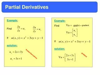
15. PARTIAL DERIVATIVES. PARTIAL DERIVATIVES. One of the most important ideas in single-variable calculus is: As we zoom in toward a point on the graph of a differentiable function, the graph becomes indistinguishable from its tangent line.


PARTIAL DERIVATIVES
E N D
Presentation Transcript
15 PARTIAL DERIVATIVES
PARTIAL DERIVATIVES • One of the most important ideas in single-variable calculus is: • As we zoom in toward a point on the graph of a differentiable function, the graph becomes indistinguishable from its tangent line. • We can then approximate the function by a linear function.
PARTIAL DERIVATIVES • Here, we develop similar ideas in three dimensions. • As we zoom in toward a point on a surface that is the graph of a differentiable function of two variables, the surface looks more and more like a plane (its tangent plane). • We can then approximate the function by a linear function of two variables.
PARTIAL DERIVATIVES • We also extend the idea of a differential to functions of two or more variables.
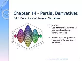
PARTIAL DERIVATIVES 15.4Tangent Planes and Linear Approximations • In this section, we will learn how to: • Approximate functions using • tangent planes and linear functions.
TANGENT PLANES • Suppose a surface S has equation z = f(x, y), where f has continuous first partial derivatives. • Let P(x0, y0, z0) be a point on S.
TANGENT PLANES • As in Section 15.3, let C1 and C2 be the curves obtained by intersecting the vertical planes y = y0 and x = x0 with the surface S. • Then, the point Plies on both C1 and C2. Fig. 15.4.1, p. 928
TANGENT PLANES • Let T1 and T2 be the tangent lines to the curves C1 and C2 at the point P. Fig. 15.4.1, p. 928
TANGENT PLANE • Then, the tangent planeto the surface Sat the point P is defined to be the plane that contains both tangent lines T1 and T2. Fig. 15.4.1, p. 928
TANGENT PLANES • We will see in Section 15.6 that, if C is any other curve that lies on the surface Sand passes through P, then its tangent line at P also lies in the tangent plane.
TANGENT PLANES • Therefore, you can think of the tangent plane to S at P as consisting of all possible tangent lines at P to curves that lie on S and pass through P. • The tangent plane at P is the plane that most closely approximates the surface Snear the point P.
TANGENT PLANES • We know from Equation 7 in Section 13.5 that any plane passing through the point P(x0, y0, z0) has an equation of the form • A(x – x0) + B(y – y0) + C(z – z0) = 0
TANGENT PLANES Equation 1 • By dividing that equation by C and letting a = –A/C and b = –B/C, we can write it in the form • z – z0 = a(x – x0) + b(y – y0)
TANGENT PLANES • If Equation 1 represents the tangent plane at P, then its intersection with the plane y = y0 must be the tangent line T1.
TANGENT PLANES • Setting y = y0 in Equation 1 gives: • z – z0 = a(x – x0) y = y0 • We recognize these as the equations (in point-slope form) of a line with slope a.
TANGENT PLANES • However, from Section 15.3, we know that the slope of the tangent T1 is fx(x0, y0). • Therefore, a = fx(x0, y0).
TANGENT PLANES • Similarly, putting x = x0 in Equation 1, we get: z – z0 = b(y – y0) • This must represent the tangent line T2. • Thus, b = fy(x0, y0).
TANGENT PLANES Equation 2 • Suppose f has continuous partial derivatives. • An equation of the tangent plane to the surface z = f(x, y) at the point P(x0, y0, z0) is: • z –z0 = fx(x0, y0)(x –x0) + fy(x0, y0)(y –y0)
TANGENT PLANES Example 1 • Find the tangent plane to the elliptic paraboloid z = 2x2 + y2 at the point (1, 1, 3). • Let f(x, y) = 2x2 + y2. • Then, fx(x, y) = 4xfy(x, y) = 2y fx(1, 1) = 4 fy(1, 1) = 2
TANGENT PLANES Example 1 • So, Equation 2 gives the equation of the tangent plane at (1, 1, 3) as: z – 3 = 4(x – 1) + 2(y – 1) or z = 4x + 2y – 3
TANGENT PLANES • The figure shows the elliptic paraboloid and its tangent plane at (1, 1, 3) that we found in Example 1. Fig. 15.4.2a, p. 929
TANGENT PLANES • Here, we zoom in toward the point by restricting the domain of the function f(x, y) = 2x2 + y2. Fig. 15.4.2a, b, p. 929
TANGENT PLANES • Notice that, the more we zoom in, • The flatter the graph appears. • The more it resembles its tangent plane. Fig. 15.4.2, p. 929
TANGENT PLANES • Here, we corroborate that impression by zooming in toward the point (1, 1) on a contour map of the function f(x, y) = 2x2 + y2. Fig. 15.4.3, p. 929
TANGENT PLANES • Notice that, the more we zoom in, the more the level curves look like equally spaced parallel lines—characteristic of a plane. Fig. 15.4.3, p. 929
LINEAR APPROXIMATIONS • In Example 1, we found that an equation of the tangent plane to the graph of the function f(x, y) = 2x2 + y2 at the point (1, 1, 3) is: • z = 4x + 2y – 3
LINEAR APPROXIMATIONS • Thus, in view of the visual evidence in the previous two figures, the linear function of two variables • L(x, y) = 4x + 2y – 3 • is a good approximation to f(x, y) when (x, y) is near (1, 1).
LINEARIZATION & LINEAR APPROXIMATION • The function L is called the linearization of f at (1, 1). • The approximation f(x, y) ≈ 4x + 2y – 3 is called the linear approximation or tangent plane approximation of f at (1, 1).
LINEAR APPROXIMATIONS • For instance, at the point (1.1, 0.95), the linear approximation gives: f(1.1, 0.95) ≈ 4(1.1) + 2(0.95) – 3 = 3.3 • This is quite close to the true value of f(1.1, 0.95) = 2(1.1)2 + (0.95)2 = 3.3225
LINEAR APPROXIMATIONS • However, if we take a point farther away from (1, 1), such as (2, 3), we no longer get a good approximation. • In fact, L(2, 3) = 11, whereas f(2, 3) = 17.
LINEAR APPROXIMATIONS • In general, we know from Equation 2 that an equation of the tangent plane to the graph of a function f of two variables at the point (a, b, f(a, b)) is: • z = f(a, b) + fx(a, b)(x – a) + fy(a, b)(y – b)
LINEARIZATION Equation 3 • The linear function whose graph is this tangent plane, namely • L(x, y) = f(a, b) + fx(a, b)(x – a) + fy(a, b)(y – b) • is called the linearization of f at (a, b).
LINEAR APPROXIMATION Equation 4 • The approximation • f(x, y) ≈f(a, b) + fx(a, b)(x – a) + fy(a, b)(y – b) • is called the linear approximation or the tangent plane approximation of f at (a, b).
LINEAR APPROXIMATIONS • We have defined tangent planes for surfaces z = f(x, y), where f has continuous first partial derivatives. • What happens if fx and fy are not continuous?
LINEAR APPROXIMATIONS • The figure pictures such a function. • Its equation is: Fig. 15.4.4, p. 930
LINEAR APPROXIMATIONS • You can verify (see Exercise 46) that its partial derivatives exist at the origin and, in fact, fx(0, 0) = 0 and fy(0, 0) = 0. • However, fx and fy are not continuous.
LINEAR APPROXIMATIONS • Thus, the linear approximation would be f(x, y) ≈ 0. • However, f(x, y) = ½ at all points on the line y = x.
LINEAR APPROXIMATIONS • Thus, a function of two variables can behave badly even though both of its partial derivatives exist. • To rule out such behavior, we formulate the idea of a differentiable function of two variables.
LINEAR APPROXIMATIONS • Recall that, for a function of one variable, y = f(x), if x changes from a to a + ∆x, we defined the increment of y as: • ∆y = f(a + ∆x) – f(a)
LINEAR APPROXIMATIONS Equation 5 • In Chapter 3 we showed that, if f is differentiable at a, then ∆y = f’(a)∆x + ε∆xwhere ε → 0 as ∆x → 0
LINEAR APPROXIMATIONS • Now, consider a function of two variables, z = f(x, y). • Suppose x changes from a to a + ∆xand y changes from b to b + ∆x.
LINEAR APPROXIMATIONS Equation 6 • Then, the corresponding increment of z is: • ∆z =f(a + ∆x, b + ∆y) – f(a, b)
LINEAR APPROXIMATIONS • Thus, the increment ∆zrepresents the change in the value of f when (x, y) changes from (a, b) to (a + ∆x, b + ∆y). • By analogy with Equation 5, we define the differentiability of a function of two variables as follows.
LINEAR APPROXIMATIONS Definition 7 • If z = f(x, y), then f is differentiable at (a, b) if ∆z can be expressed in the form • ∆z = fx(a, b) ∆x + fy(a, b) ∆y + ε1 ∆x + ε2 ∆y • where ε1 and ε2 → 0 as (∆x, ∆y) → (0, 0).
LINEAR APPROXIMATIONS • Definition 7 says that a differentiable function is one for which the linear approximation in Equation 4 is a good approximation when (x, y) is near (a, b). • That is, the tangent plane approximates the graph of f well near the point of tangency.
LINEAR APPROXIMATIONS • It’s sometimes hard to use Definition 7 directly to check the differentiability of a function. • However, the next theorem provides a convenient sufficient condition for differentiability.
LINEAR APPROXIMATIONS Theorem 8 • If the partial derivatives fx and fy exist near (a, b) and are continuous at (a, b), then f is differentiable at (a, b).
LINEAR APPROXIMATIONS Example 2 • Show that f(x, y) = xexy is differentiable at (1, 0) and find its linearization there. • Then, use it to approximate f(1.1, –0.1).
LINEAR APPROXIMATIONS Example 2 • The partial derivatives are: • fx(x, y) = exy + xyexyfy(x, y) = x2exy fx(1, 0) = 1 fy(1, 0) = 1 • Both fx and fy are continuous functions. • So, f is differentiable by Theorem 8.
LINEAR APPROXIMATIONS Example 2 • The linearization is: • L(x, y) = f(1, 0) + fx(1, 0)(x – 1) + fy(1, 0)(y – 0) • = 1 + 1(x – 1) + 1 .y = x + y Fig. 15.4.5, p. 931