Download
1 / 35
350 likes | 482 Views
If your several predictors are categorical , MRA is identical to ANOVA. If your sole predictor is continuous , MRA is identical to correlational analysis. If your sole predictor is dichotomous , MRA is identical to a t-test. Do your residuals meet the required assumptions ?.

E N D
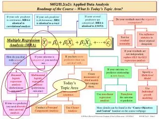
If your several predictors are categorical, MRA is identical to ANOVA If your sole predictor is continuous, MRA is identical to correlational analysis If your solepredictor is dichotomous, MRA is identical to a t-test Do your residuals meet the required assumptions? Use influence statistics to detect atypical datapoints Test for residual normality Multiple Regression Analysis (MRA) If your residuals are not independent, replace OLS byGLS regression analysis If you have more predictors than you can deal with, If your outcome is categorical, you need to use… How do you deal with missing data? If your outcome vs. predictor relationship isnon-linear, Specify a Multi-level Model Create taxonomies of fitted models and compare them. Binomiallogistic regression analysis (dichotomous outcome) Multinomial logistic regression analysis (polytomous outcome) Today’s Topic Area Form composites of the indicators of any common construct. Use Individual growth modeling Use non-linear regression analysis. Transform the outcome or predictor If time is a predictor, you need discrete-time survival analysis… Conduct a Principal Components Analysis Use Cluster Analysis More details can be found in the “Course Objectives and Content” handout on the course webpage. S052/II.2(a2): Applied Data AnalysisRoadmap of the Course – What Is Today’s Topic Area?
Today, in the second part of Syllabus Section II.2(a), onDiscrete-Time Survival Analysis, I will: • Replicate life-table analyses by conducting logistic regression analyses of EVENT as a function of PERIOD in the person-period dataset, using a general specification for PERIOD (Slides#4 - #17). • Show how the completely general specification for PERIOD can be represented in a useful “no intercept” version (Slides #18 - #23). • Appendix 1 compares the “intercept” and “no intercept” specifications of the DTSA model algebraically (Slide #24). • Appendix 2 demonstrates the arithmetic equivalence of the “intercept” and “no intercept” specifications (Slide #25). • Appendix 3 shows how the general specification of PERIOD can be replaced by more parsimonious polynomial specifications (Slides #26 - #35). S052/II.2(a2): Introducing Discrete-Time Survival Analysis Printed Syllabus – What Is Today’s Topic? Please check inter-connections among the Roadmap, the Daily Topic Area, the Printed Syllabus, and the content of today’s class when you pre-read the day’s materials.
Classical Methods of Survival Analysis • Simple data-analytic approaches for summarizing survival data appropriately: • Estimation of the sample hazard function. • Estimation of the sample survivor function. • Estimation of the median lifetime. • Simple tests of differences in survivor function, by “group”: • Survival analytic equivalent of the t-test. Discrete-Time Survival Analysis • Easily replicates classical methods of survival analysis, using logistic regression analysis. • Reframes classical survival analytic methods in a regression format: • Permits the inclusion of multiple predictors, including interactions. • Provides testing with the Wald test & differences in the –2LL statistic. • Fitted hazard & survivor functions, & median lifetimes, are easily recovered from the fitted logistic model. Continuous-Time Survival Analysis • A replacement for discrete-time survival analysis when time has been measured continuously. • Imposes additional assumptions on the data. • Reframes classical survival analytic methods in a regression format: • Permits the inclusion of predictors, including interactions. • Accompanied by its own testing procedures, based on standard practices. • Fitted hazard & survivor functions, & median lifetimes, are easily recovered from fitted models. Last Time Today, & Next Time Next year, … ? S052/II.2(a2): Introducing Discrete-Time Survival Analysis Three Kinds Of Survival Analysis
In order to proceed, let’s continue to work in the person-period dataset and with the new summary statistics I have introduced: • Hazard probability& the hazard function. • Survival probability & the survivor function. • Median lifetime. • But, let’s use logistic regression analysis to model & estimate them .. S052/II.2(a2): Introducing Discrete-Time Survival Analysis The Person-Period Dataset for the Special Educator Data
The earlier YRSTCH variable, which recorded the duration of the teaching career in the person-level dataset, has been replaced by variable PERIOD, which labels the time-period to which each row of the person-period dataset refers. The person-period dataset contains other variables too, that are labeled and explained in these rows of the codebook. We will incorporate these variables into the analysis in today’s presentation. We’ve also acquired a new variable called EVENT, which records whether a teacher experienced the event of interest (“quit teaching”) in the particular discrete time-period in question Recall that, in theperson-period datasetfrom the previous class, each teacher hasone row of data for each year of their career, and that each row contains the following information … S052/II.2(a2): Introducing Discrete-Time Survival Analysis The Person-Period Dataset for the Special Educator Data
Notice how, in the person-period dataset, outcome EVENT has been encoded to embody the same conditionality present in the definition of the hazard probability … In our earlier life-table analysis in the person-period dataset: • EVENT recorded whether the teacher experienced the event of interest (quitting teaching) in each timePERIOD. • Conceptually, in these analyses: • EVENT served as a (dichotomous)outcome. • PERIOD served as a predictor. In a person-period dataset: • Each person has one row of data in each time-period. • Their data record continues until, and includes, the time-period in which theyexperience theevent of interest, or arecensored: • A person cannot be present in a time-period unless they had a value of 0 for EVENT in the previous period. • In other words, they must have survived the prior period. • So, the person-period dataset has been formatted to permiteach person to be present in a particular time periodonly if they are a legitimate member of the risk set in that period. So, why not replace life table analysis by the logistic regression analysis ofEVENTonPERIODin theperson-period dataset? • From a technical perspective, this turns out to be exactly the right thing to do. • It’s then called Discrete-Time Survival Analysis. Person-Period Dataset ID PERIOD EVENT 1 1 1 2 1 0 2 2 1 3 1 1 4 1 1 5 1 0 5 2 0 5 3 0 5 4 0 5 5 0 5 6 0 5 7 0 5 8 0 5 9 0 5 10 0 5 11 0 5 12 0 6 1 1 7 1 0 7 2 0 7 3 0 7 4 0 7 5 0 7 6 0 7 7 0 7 8 0 7 9 0 7 10 0 7 11 0 7 12 0 Etc. S052/II.2(a2): Introducing Discrete-Time Survival Analysis The Person-Period Dataset for the Special Educator Data
Dichotomous predictors, P1 thru P12 are defined to distinguish among the discrete time periods. • For each person in each period, each of the time period indicators, P1 thru P12, is set to 1 in the corresponding period, and 0 in other periods. Representing PERIOD by these time indicators in our logistic regression analysis provides themost general specificationpossible for any potential relationship between EVENT andPERIOD. To conduct logistic regression analyses in the person-period dataset, we must think about how we represent time PERIOD in our models -- recall that the dataset contains a vector of predictors that we have not yet used … S052/II.2(a2): Introducing Discrete-Time Survival Analysis The Most General Way of Specifying Time PERIOD That Is Possible?
ID EVENT PERIOD P1 P2 P3 P4 P5 P6 P7 P8 P9 P10 P11 P12 1 Quit 1 1 0 0 0 0 0 0 0 0 0 0 0 2 No Quit 1 1 0 0 0 0 0 0 0 0 0 0 0 2 Quit 2 0 1 0 0 0 0 0 0 0 0 0 0 3 Quit 1 1 0 0 0 0 0 0 0 0 0 0 0 4 Quit 1 1 0 0 0 0 0 0 0 0 0 0 0 5 No Quit 1 1 0 0 0 0 0 0 0 0 0 0 0 5 No Quit 2 0 1 0 0 0 0 0 0 0 0 0 0 5 No Quit 3 0 0 1 0 0 0 0 0 0 0 0 0 5 No Quit 4 0 0 0 1 0 0 0 0 0 0 0 0 5 No Quit 5 0 0 0 0 1 0 0 0 0 0 0 0 5 No Quit 6 0 0 0 0 0 1 0 0 0 0 0 0 5 No Quit 7 0 0 0 0 0 0 1 0 0 0 0 0 5 No Quit 8 0 0 0 0 0 0 0 1 0 0 0 0 5 No Quit 9 0 0 0 0 0 0 0 0 1 0 0 0 5 No Quit 10 0 0 0 0 0 0 0 0 0 1 0 0 5 No Quit 11 0 0 0 0 0 0 0 0 0 0 1 0 5 No Quit 12 0 0 0 0 0 0 0 0 0 0 0 1 6 Quit 1 1 0 0 0 0 0 0 0 0 0 0 0 Here’s the original 12 years of data on the time periods in which Teacher #5 was present in the person-period dataset The time-period indicators, P1 - P12, identify each time-period in a very general way In the 1st time period: • P1= 1 • P2 thru P12 = 0 In the 2nd time period: • P2= 1 • P1 & P3 thru P12= 0 In the 12th time period: • P12= 1, • P1 thru P11 = 0. … Here I have printed out the values of the time-period indicators for a few folk from the person-period dataset … S052/II.2(a2): Introducing Discrete-Time Survival Analysis The Most General Way of Specifying Time PERIOD That Is Possible?
Here are the time-period indicators -- P1 through P12 -- that were present in the person-period dataset, but were input and ignored up to this point. Here I list the values of EVENT and P1 thru P12 for the few cases we inspected on the previous slide. Here, I specify EVENT as a logistic function of time-period indicators, P2 thru P12,and fit the model in the person-period dataset: • I have omitted onetime-period indicator, by choice – here, P1 – as usual, to avoidcompletemulti-collinearity among them all. • As with dichotomous predictors in any analysis, the omission of one dummy predictor defines a “reference category” for interpretation later. • The hypothesized probability of event occurrence for the ith person, in the jth time-period, is then: Here I output predicted values, PREDQUIT1, into a newdataset called PREDICTED1, to facilitate subsequent listing of the fitted hazard probabilities and plotting of the fitted hazard function. Here’s the SAS code for Data-Analytic Handout II.2(a).3, in which I conduct the suggested logistic regression analyses of EVENT for the first time … DATA SPEC_ED_PP; INFILE 'C:\DATA\S052\SPEC_ED_PP.txt'; INPUT ID PERIOD EVENT P1-P12; LABEL ID = 'Teacher Identification Code' PERIOD = 'Current Time Period' EVENT = 'Did Teacher Quit in this Time Period?'; PROCFORMAT; VALUE EFMT 0='No Quit' 1='Quit'; * Print first 33 rows from the person-period dataset, to reveal the coding of time period dummies, P1-P12; PROCPRINT DATA=SPEC_ED_PP(OBS=33); VAR ID EVENT PERIOD P1-P12; FORMAT EVENT EFMT.; * Predict event occurrence ("quitting teaching") by P2-P12; PROCLOGISTIC DATA=SPEC_ED_PP; MODEL EVENT(event='Quit') = P2-P12; FORMAT EVENT EFMT.; OUTPUT OUT=PREDICTED1 PREDICTED=PREDQUIT1; S052/II.2(a2): Introducing Discrete-Time Survival Analysis Fitting the First DTSA Model, Using the Most General Specification for PERIOD
We reject the H0 that the time-period indicators, P2 thru P12,have no joint effect on EVENT, in the population (p<.0001). Notice that the current model contains time-period indicators, P2 thru P12,as predictors Here’s the fitted logistic regression model … interpreting the associated hypothesis tests is straightforward! Model Fit Statistics: Intercept only, -2LL = 14903.8 Intercept & covariates, -2LL = 14583.7 Difference in –2LL = 320.1 Model Fit Statistics Intercept Intercept and Criterion Only Covariates -2 Log L 14903.844 14583.742 Testing Global Null Hypothesis: BETA=0 Test Chi-Square DF Pr > ChiSq Likelihood Ratio 320.1019 11 <.0001 Analysis of Maximum Likelihood Estimates Standard Wald Parameter Estimate Error Chi-Square Pr > ChiSq Intercept -2.0337 0.0498 1667.8155 <.0001 P2 -0.0551 0.0735 0.5617 0.4536 P3 0.000610 0.0750 0.0001 0.9935 P4 -0.0819 0.0792 1.0687 0.3012 P5 -0.2911 0.0867 11.2736 0.0008 P6 -0.3745 0.0917 16.6879 <.0001 P7 -0.7152 0.1055 45.9575 <.0001 P8 -0.9512 0.1256 57.3427 <.0001 P9 -1.0886 0.1489 53.4261 <.0001 P10 -1.2277 0.1793 46.8833 <.0001 P11 -1.6425 0.2580 40.5338 <.0001 P12 -2.3104 0.4524 26.0867 <.0001 S052/II.2(a2): Introducing Discrete-Time Survival Analysis Fitting the First DTSA Model, Using the Most General Specification for PERIOD Using this difference in –2LL statistic between unconditional and current models, we can test the null hypothesis that time period indicators, P2 thru P12, have no joint effect on EVENT, in the population.
To compute fitted probability of quitting teachinginTIME PERIOD #1, I set all included time-period indicators -- P2thruP12 -- to a value of 0, as follows: Fitted hazard probability in time period #1: Fitted values of the outcome are obtained as usual by substituting predictor values into the fitted model .. Model Fit Statistics Intercept Intercept and Criterion Only Covariates -2 Log L 14903.844 14583.742 Testing Global Null Hypothesis: BETA=0 Test Chi-Square DF Pr > ChiSq Likelihood Ratio 320.1019 11 <.0001 Analysis of Maximum Likelihood Estimates Standard Wald Parameter Estimate Error Chi-Square Pr > ChiSq Intercept -2.0337 0.0498 1667.8155 <.0001 P2 -0.0551 0.0735 0.5617 0.4536 P3 0.000610 0.0750 0.0001 0.9935 P4 -0.0819 0.0792 1.0687 0.3012 P5 -0.2911 0.0867 11.2736 0.0008 P6 -0.3745 0.0917 16.6879 <.0001 P7 -0.7152 0.1055 45.9575 <.0001 P8 -0.9512 0.1256 57.3427 <.0001 P9 -1.0886 0.1489 53.4261 <.0001 P10 -1.2277 0.1793 46.8833 <.0001 P11 -1.6425 0.2580 40.5338 <.0001 P12 -2.3104 0.4524 26.0867 <.0001 S052/II.2(a2): Introducing Discrete-Time Survival Analysis Fitting the First DTSA Model, Using the Most General Specification for PERIOD
To compute fitted probability of quitting teachinginTIME PERIOD #2, I set time-period indicator P2 to 1, and the rest of the indicators to 0, as follows: Fitted hazard probability in time period #2: Fitted values of the outcome are obtained by substituting predictor values into the fitted model, as usual! Model Fit Statistics Intercept Intercept and Criterion Only Covariates -2 Log L 14903.844 14583.742 Testing Global Null Hypothesis: BETA=0 Test Chi-Square DF Pr > ChiSq Likelihood Ratio 320.1019 11 <.0001 Analysis of Maximum Likelihood Estimates Standard Wald Parameter Estimate Error Chi-Square Pr > ChiSq Intercept -2.0337 0.0498 1667.8155 <.0001 P2 -0.0551 0.0735 0.5617 0.4536 P3 0.000610 0.0750 0.0001 0.9935 P4 -0.0819 0.0792 1.0687 0.3012 P5 -0.2911 0.0867 11.2736 0.0008 P6 -0.3745 0.0917 16.6879 <.0001 P7 -0.7152 0.1055 45.9575 <.0001 P8 -0.9512 0.1256 57.3427 <.0001 P9 -1.0886 0.1489 53.4261 <.0001 P10 -1.2277 0.1793 46.8833 <.0001 P11 -1.6425 0.2580 40.5338 <.0001 P12 -2.3104 0.4524 26.0867 <.0001 S052/II.2(a2): Introducing Discrete-Time Survival Analysis Fitting the First DTSA Model, Using the Most General Specification for PERIOD
To compute fitted probability of quitting teachingintheTIME PERIOD #3, I set time-period indicator P3 to 1, and the rest of the indicators to 0, as follows: Fitted hazard probability for time period #3: Fitted values of the outcome are obtained by substituting predictor values into the fitted model, as usual! Model Fit Statistics Intercept Intercept and Criterion Only Covariates -2 Log L 14903.844 14583.742 Testing Global Null Hypothesis: BETA=0 Test Chi-Square DF Pr > ChiSq Likelihood Ratio 320.1019 11 <.0001 Analysis of Maximum Likelihood Estimates Standard Wald Parameter Estimate Error Chi-Square Pr > ChiSq Intercept -2.0337 0.0498 1667.8155 <.0001 P2 -0.0551 0.0735 0.5617 0.4536 P3 0.000610 0.0750 0.0001 0.9935 P4 -0.0819 0.0792 1.0687 0.3012 P5 -0.2911 0.0867 11.2736 0.0008 P6 -0.3745 0.0917 16.6879 <.0001 P7 -0.7152 0.1055 45.9575 <.0001 P8 -0.9512 0.1256 57.3427 <.0001 P9 -1.0886 0.1489 53.4261 <.0001 P10 -1.2277 0.1793 46.8833 <.0001 P11 -1.6425 0.2580 40.5338 <.0001 P12 -2.3104 0.4524 26.0867 <.0001 S052/II.2(a2): Introducing Discrete-Time Survival Analysis Fitting the First DTSA Model, Using the Most General Specification for PERIOD Etc. … Of course, you don’t need to do these calculations yourself … you can use the predicted values!
Here’s standard output of predicted values, PREDQUIT1, into a new dataset called PREDICTED1, to facilitate subsequent listing of the fitted hazard probabilities and plotting of the fitted hazard function. Here, I sort the predicted values by time-period, picking out the first value listed in each time period. List the fitted values for inspection. These turn out to be the fitted hazard probabilities. Plot the fitted values versus time-period. This turnd out to be the fitted hazard function. PC-SAS code for obtaining, inspecting & plotting the predicted values in each of the discrete time periods … * Predict event occurrence ("quitting teaching") by P2-P12; PROC LOGISTIC DATA=SPEC_ED_PP; MODEL EVENT(event='Quit') = P2-P12; FORMAT EVENT EFMT.; OUTPUT OUT=PREDICTED1 PREDICTED=PREDQUIT1; * Re-sort output dataset and pick out the 12 unique values of predicted hazard probability, one per discrete time period; PROC SORT DATA=PREDICTED1; BY PERIOD; DATA PREDICTED1; SET PREDICTED1; BY PERIOD; IF FIRST.PERIOD=1; * List & plot the unique predicted hazard probabilities, one/discrete period; PROC PRINT DATA=PREDICTED1; VAR PERIOD PREDQUIT1; PROC PLOT DATA=PREDICTED1; PLOT PREDQUIT1*PERIOD='P' / VAXIS=0 TO .14 BY .02 HAXIS=0 TO 13 BY 1; S052/II.2(a2): Introducing Discrete-Time Survival Analysis Obtaining, Inspecting and Plotting Fitted Hazard Probabilities Automatically
And here are the sample hazard probabilities, from the life-table analysis EVENT(Did Teacher Quit in this Time Period?) Frequency‚ Col Pct ‚ 1‚ 2‚ 3‚ 4‚ 5‚ 6‚ ƒƒƒƒƒƒƒƒƒˆƒƒƒƒƒƒƒƒˆƒƒƒƒƒƒƒƒˆƒƒƒƒƒƒƒƒˆƒƒƒƒƒƒƒƒˆƒƒƒƒƒƒƒƒˆƒƒƒƒƒƒƒƒˆ No Quit ‚ 3485 ‚ 3101 ‚ 2742 ‚ 2447 ‚ 2229 ‚ 2045 ‚ ‚ 88.43 ‚ 88.98 ‚ 88.42 ‚ 89.24 ‚ 91.09 ‚ 91.75 ‚ ƒƒƒƒƒƒƒƒƒˆƒƒƒƒƒƒƒƒˆƒƒƒƒƒƒƒƒˆƒƒƒƒƒƒƒƒˆƒƒƒƒƒƒƒƒˆƒƒƒƒƒƒƒƒˆƒƒƒƒƒƒƒƒˆ Quit ‚ 456‚ 384 ‚ 359 ‚ 295 ‚ 218 ‚ 184 ‚ ‚11.57‚ 11.02 ‚ 11.58 ‚ 10.76 ‚ 8.91 ‚ 8.25‚ ƒƒƒƒƒƒƒƒƒˆƒƒƒƒƒƒƒƒˆƒƒƒƒƒƒƒƒˆƒƒƒƒƒƒƒƒˆƒƒƒƒƒƒƒƒˆƒƒƒƒƒƒƒƒˆƒƒƒƒƒƒƒƒˆTotal 3941 3485 3101 2742 2447 2229 PERIOD(Current Time Period) ‚ 7‚ 8‚ 9‚ 10‚ 11‚ 12‚ Total ˆƒƒƒƒƒƒƒƒˆƒƒƒƒƒƒƒƒˆƒƒƒƒƒƒƒƒˆƒƒƒƒƒƒƒƒˆƒƒƒƒƒƒƒƒˆƒƒƒƒƒƒƒƒˆ ‚ 1922 ‚ 1563 ‚ 1203 ‚ 913 ‚ 632 ‚ 386 ‚ 22668 ‚ 93.99 ‚ 95.19 ‚ 95.78 ‚ 96.31 ‚ 97.53 ‚ 98.72 ‚ ˆƒƒƒƒƒƒƒƒˆƒƒƒƒƒƒƒƒˆƒƒƒƒƒƒƒƒˆƒƒƒƒƒƒƒƒˆƒƒƒƒƒƒƒƒˆƒƒƒƒƒƒƒƒˆ ‚ 123 ‚ 79 ‚ 53 ‚ 35 ‚ 16 ‚ 5 ‚ 2207 ‚6.01 ‚ 4.81 ‚ 4.22 ‚ 3.69 ‚ 2.47 ‚ 1.28‚ ˆƒƒƒƒƒƒƒƒˆƒƒƒƒƒƒƒƒˆƒƒƒƒƒƒƒƒˆƒƒƒƒƒƒƒƒˆƒƒƒƒƒƒƒƒˆƒƒƒƒƒƒƒƒˆ 2045 1642 1256 948 648 391 24875 Here are the fitted probabilities, direct from the PC-SAS output … PERIOD PREDQUIT1 1 0.11571 2 0.11019 3 0.11577 4 0.10759 5 0.08909 6 0.08255 7 0.06015 8 0.04811 9 0.04220 10 0.03692 11 0.02469 12 0.01282 S052/II.2(a2): Introducing Discrete-Time Survival Analysis Inspecting the Fitted Probabilities by PERIOD Notice that the fitted probabilities obtained in the logistic regression analysis are identical to the sample hazard probabilities obtained in the life table analysis …
Notice that the fitted probabilities from the logistic regression analysis provide the same sample hazard function that we obtained in the life table analysis And, here are the fitted probabilities plotted versus time period, from the PC-SAS output … Fitted Hazard Function Most General Specification of PERIOD 0.14 ˆ ‚ ‚ ‚ E 0.12 ˆ s ‚ P P t ‚ P P i ‚ m 0.10 ˆ a ‚ t ‚ P e ‚ P d 0.08 ˆ ‚ P ‚ r ‚ o 0.06 ˆ P b ‚ a ‚ P b ‚ i 0.04 ˆ P l ‚ P i ‚ t ‚ P y 0.02 ˆ ‚ P ‚ ‚ 0.00 ˆ Šƒˆƒƒƒƒˆƒƒƒƒˆƒƒƒƒˆƒƒƒƒˆƒƒƒƒˆƒƒƒƒˆƒƒƒƒˆƒƒƒƒˆƒƒƒƒˆƒƒƒƒˆƒƒƒƒˆƒƒƒƒˆƒƒƒƒˆƒƒ 0 1 2 3 4 5 6 7 8 9 10 11 12 13 Current Time Period PERIOD PREDQUIT1 1 0.11571 2 0.11019 3 0.11577 4 0.10759 5 0.08909 6 0.08255 7 0.06015 8 0.04811 9 0.04220 10 0.03692 11 0.02469 12 0.01282 S052/II.2(a2): Introducing Discrete-Time Survival Analysis Fitted Hazard Probabilities vs. PERIOD We conclude that we canreplicate life-table analysisby conductinglogistic regression analyses in the person-period dataset … we refer to this asDiscrete-Time Survival Analysis.
Once you’ve estimated the fitted hazard probabilitiesin each time period, you canplot the hazard functionand, from it,estimatethefitted survivor functionandmedian lifetimein the usual way … S052/II.2(a2): Introducing Discrete-Time Survival Analysis Finishing The Job – Fitted Survivor Function & Median Lifetime Statistic 6.6 years
Notice you can regress EVENT on all the time-period dummies, P1 thru P12, by dropping the intercept from the model: • Notice the “NOINT” option. • Omission of the intercept parameter changes the interpretation of the parameters associated with the time-dummies, but the new interpretation is very useful! • The new discrete-time hazard model, for the ith person on the jth occasion, is then: Here are the usual listing and bivariate plot of the fitted (hazard) probabilities versus time-period. Usefully, you can specify the discrete-time hazard model in another equivalent way… with “no intercept” * Predict event occurrence ("quitting teaching") again by time-period dummies, but avoid collinearity by retaining all time-period dummies & dropping intercept; PROCLOGISTIC DATA=SPEC_ED_PP; MODEL EVENT(event='Quit') = P1-P12 / NOINT ; FORMAT EVENT EFMT.; OUTPUT OUT=PREDICTED2 PREDICTED=PREDQUIT2; * Re-sort output dataset and pick out the twelve unique values of predicted hazard probability, one per discrete time period; PROCSORT DATA=PREDICTED2; BY PERIOD; DATA PREDICTED2; SET PREDICTED2; BY PERIOD; IF FIRST.PERIOD=1; * List & plot the unique predicted hazard probabilities, one per discrete period; PROCPRINT DATA=PREDICTED2; VAR PERIOD PREDQUIT2; PROCPLOT DATA=PREDICTED2; PLOT PREDQUIT2*PERIOD='P' / VAXIS=0 TO .14 BY .02 HAXIS=0 TO 13 BY 1; S052/II.2(a2): Introducing Discrete-Time Survival Analysis An Interesting Alternative General Specification of PERIOD, This Time With “No Intercept”
The-2LL statistic for this model is identical to its earlier value in the general “intercept” specification. Why? Because now a comparison of model -2LLstatistics is testing the null hypothesis that “all hazard probabilities are jointly equal to zero” in the population, rather than “all hazard probabilities are jointly equal to the hazard probability in time period #1” (Appendix I). Notice the current model contains all the time-period indicators, P1 thru P12,as predictors But, the difference in the-2LL statistic between the unconditional and current models is not thesame as the value obtained under the “intercept” specification. Model Fit Statistics Without With Criterion Covariates Covariates -2 Log L 34484.072 14583.742 Testing Global Null Hypothesis: BETA=0 Test Chi-Square DF Pr > ChiSq Likelihood Ratio 19900.3302 12 <.0001 Analysis of Maximum Likelihood Estimates Standard Wald Parameter Estimate Error Chi-Square Pr > ChiSq P1 -2.0337 0.0498 1667.8155 <.0001 P2 -2.0888 0.0541 1490.8689 <.0001 P3 -2.0331 0.0561 1312.1587 <.0001 P4 -2.1156 0.0616 1178.3470 <.0001 P5 -2.3248 0.0710 1073.2694 <.0001 P6 -2.4082 0.0770 979.0219 <.0001 P7 -2.7489 0.0930 873.5642 <.0001 P8 -2.9849 0.1153 670.0029 <.0001 P9 -3.1223 0.1404 494.8756 <.0001 P10 -3.2614 0.1722 358.5382 <.0001 P11 -3.6763 0.2531 210.9037 <.0001 P12 -4.3464 0.4501 93.2502 <.0001 S052/II.2(a2): Introducing Discrete-Time Survival Analysis An Interesting Alternative General Specification of PERIOD, This Time With “No Intercept”
To compute fitted probability of quitting teachingintime period #1, I set time indicator P1 to 1 and all other time indicators to 0, as follows: Fitted hazard probability in time period #1: • Identical to the value obtained in earlier life table and discrete-time survival analyses. Under the general “no intercept” specification for PERIOD, the recovery of the fitted hazard probabilities in each time period is simpler … here’s the computation of thefitted hazard probabilityintime period #1… Model Fit Statistics Without With Criterion Covariates Covariates -2 Log L 34484.072 14583.742 Testing Global Null Hypothesis: BETA=0 Test Chi-Square DF Pr > ChiSq Likelihood Ratio 19900.3302 12 <.0001 Analysis of Maximum Likelihood Estimates Standard Wald Parameter Estimate Error Chi-Square Pr > ChiSq P1 -2.0337 0.0498 1667.8155 <.0001 P2 -2.0888 0.0541 1490.8689 <.0001 P3 -2.0331 0.0561 1312.1587 <.0001 P4 -2.1156 0.0616 1178.3470 <.0001 P5 -2.3248 0.0710 1073.2694 <.0001 P6 -2.4082 0.0770 979.0219 <.0001 P7 -2.7489 0.0930 873.5642 <.0001 P8 -2.9849 0.1153 670.0029 <.0001 P9 -3.1223 0.1404 494.8756 <.0001 P10 -3.2614 0.1722 358.5382 <.0001 P11 -3.6763 0.2531 210.9037 <.0001 P12 -4.3464 0.4501 93.2502 <.0001 S052/II.2(a2): Introducing Discrete-Time Survival Analysis An Interesting Alternative General Specification of PERIOD, This Time With “No Intercept”
To compute fitted probability of quitting teachingintime period #2, I set time indicator P2 to 1 and all other time indicators to 0, as follows: Fitted hazard probability for time period #2: • Identical to the value obtained in earlier life table and discrete-time survival analyses. Here’s the computation of thefitted hazard probabilityintime period #2… Model Fit Statistics Without With Criterion Covariates Covariates -2 Log L 34484.072 14583.742 Testing Global Null Hypothesis: BETA=0 Test Chi-Square DF Pr > ChiSq Likelihood Ratio 19900.3302 12 <.0001 Analysis of Maximum Likelihood Estimates Standard Wald Parameter Estimate Error Chi-Square Pr > ChiSq P1 -2.0337 0.0498 1667.8155 <.0001 P2 -2.0888 0.0541 1490.8689 <.0001 P3 -2.0331 0.0561 1312.1587 <.0001 P4 -2.1156 0.0616 1178.3470 <.0001 P5 -2.3248 0.0710 1073.2694 <.0001 P6 -2.4082 0.0770 979.0219 <.0001 P7 -2.7489 0.0930 873.5642 <.0001 P8 -2.9849 0.1153 670.0029 <.0001 P9 -3.1223 0.1404 494.8756 <.0001 P10 -3.2614 0.1722 358.5382 <.0001 P11 -3.6763 0.2531 210.9037 <.0001 P12 -4.3464 0.4501 93.2502 <.0001 S052/II.2(a2): Introducing Discrete-Time Survival Analysis An Interesting Alternative General Specification of PERIOD, This Time With “No Intercept”
In general, with the “no intercept” specification, the fitted hazard probabilityin anytime period tj is: And the “no intercept” specification is so useful because this formula can be programmed in PC-SAS, as we will see! Here’s the computation of the fitted hazard probabilityduringtime period j… Model Fit Statistics Without With Criterion Covariates Covariates -2 Log L 34484.072 14583.742 Testing Global Null Hypothesis: BETA=0 Test Chi-Square DF Pr > ChiSq Likelihood Ratio 19900.3302 12 <.0001 Analysis of Maximum Likelihood Estimates Standard Wald Parameter Estimate Error Chi-Square Pr > ChiSq P1 -2.0337 0.0498 1667.8155 <.0001 P2 -2.0888 0.0541 1490.8689 <.0001 P3 -2.0331 0.0561 1312.1587 <.0001 P4 -2.1156 0.0616 1178.3470 <.0001 P5 -2.3248 0.0710 1073.2694 <.0001 P6 -2.4082 0.0770 979.0219 <.0001 P7 -2.7489 0.0930 873.5642 <.0001 P8 -2.9849 0.1153 670.0029 <.0001 P9 -3.1223 0.1404 494.8756 <.0001 P10 -3.2614 0.1722 358.5382 <.0001 P11 -3.6763 0.2531 210.9037 <.0001 P12 -4.3464 0.4501 93.2502 <.0001 S052/II.2(a2): Introducing Discrete-Time Survival Analysis An Interesting Alternative General Specification of PERIOD, This Time With “No Intercept”
Life table (sample) estimates of the hazard probability Sample hazard probabilities obtained from the earlier life-table analysis. Discrete-time survival analysis estimates of hazard probability, assuming a general specification of PERIOD, using time indicators P1 through P12. Predicted values of EVENT, PREDQUIT2,obtained from the no intercept specification of logistic regression model. Fitted hazard functions are identical – we can replicate life-table analysis with DTSA “no intercept” approach!!! S052/II.2(a2): Introducing Discrete-Time Survival Analysis The “Intercept” and “No Intercept” Specifications Provide the Same Hazard Function
… tests that the population values of the outcome in periods #2 through #12 are identical to the population value of the outcome in the reference period (Period #1). …… … tests that all population values of the outcome in periods #1 through #12 are zero …… Period 1 2 3 11 12 4 Log-oddsi(tj) S052/II.2(a2): Introducing Discrete-Time Survival Analysis Appendix 1: Null Hypotheses Tested Under Each Time Indicator Specification Coding of Time Period Dummies PERIOD P1 P2 P3 .. P11 P12 1 1 0 0 .. 0 0 2 0 1 0 .. 0 0 3 0 0 1 .. 0 0 4 0 0 0 .. 0 0 11 0 0 0 .. 1 0 12 0 0 0 .. 0 1 Period 1 2 3 11 12 4 Log-oddsi(tj)
Identical goodness of fit statistics Without an intercept … Model Fit Statistics Without With Covariates Covariates -2 Log L 34484.072 14583.742 Maximum Likelihood Estimates Parameter Estimate P1 -2.0337 P2 -2.0888 P3 -2.0331 P4 -2.1156 P5 -2.3248 P6 -2.4082 P7 -2.7489 P8 -2.9849 P9 -3.1223 P10 -3.2614 P11 -3.6763 P12 -4.3464 Identical estimates & identical interpretation for the fitted logit hazard associated with Time Period #1 Coeffient is the differenceinfitted logit hazard between time periods #2 & #1. Coeff is the fitted logit hazard in time period #2 = (-2.0337) + (-0.0551) -2.0888 Etc. With an intercept … Model Fit Statistics Intercept Intercept and Only Covariates -2 Log L 14903.844 14583.742 Maximum Likelihood Estimates Parameter Estimate Intercept -2.0337 P2 -0.0551 P3 0.000610 P4 -0.0819 P5 -0.2911 P6 -0.3745 P7 -0.7152 P8 -0.9512 P9 -1.0886 P10 -1.2277 P11 -1.6425 P12 -2.3104 S052/II.2(a2): Introducing Discrete-Time Survival Analysis Appendix 2: The Arithmetic Equivalence of the Two Time Indicator Specifications
Since we are investigating the relationship betweenEVENTandPERIOD, let’s not assume that it is completely general: • Let’s create some polynomial transformations of PERIOD to try out as potential predictors. • Linear, quadratic, cubic?, quartic?, etc. Print out a few cases for inspection. You can replace the general “dummy” specification by a polynomial specification, often quite successfully … I tried this several times in the back half of Data Analytic Handout II_2a_3 … *---------------------------------------------------------------------------------* Now refit the discrete-time hazard model, replacing the general specification of PERIOD -- which used the time-period dummies P1-P12 -- by more parsimonious polynomial representations of period. *---------------------------------------------------------------------------------*; DATA SPEC_ED_PP; SET SPEC_ED_PP; * Create power transformations of PERIOD, that will serve as predictors in place of time-period dummies P1-P12, in the discrete-time hazard model; * Create the square of PERIOD; PERIODSQ = PERIOD*PERIOD; * Create the square of PERIOD; PERIODCUB = PERIOD*PERIOD*PERIOD; * Could also create the quartic, quintic, etc. of PERIOD, if needed; KEEP ID PERIOD EVENT PERIODSQ PERIODCUB; * Print first few rows of person-period dataset, showing PERIOD and its corresponding power transformations; PROCPRINT DATA=SPEC_ED_PP(OBS=33); VAR ID EVENT PERIOD PERIODSQ PERIODCUB; FORMAT EVENT EFMT.; S052/II.2(a2): Introducing Discrete-Time Survival Analysis Appendix 3:Conducting DTSA Using Polynomial Functions of Period
Conduct a logistic regression analysis of EVENT on PERIOD in the person-period dataset. Regress the (log-odds of) EVENTon alinear functionof PERIOD in the usual way. Output the predicted values of EVENT– these will be the fitted hazard probabilities – here, called PREDQUIT3, into the person-period dataset. Plot the fitted probabilities of EVENT occurrenceagainst PERIOD – this provides the fitted hazard function. Print out values of the fitted hazard probability of a few cases for inspection … Here’s the discrete-time survival analyses … first, let’s use logistic regression analysis to check whether the log-odds of event occurrence is linear in PERIOD … *---------------------------------------------------------------------------------* Fit discrete-time hazard models, in which event occurrence ("quitting teaching") is predicted by polynomial functions of PERIOD of gradually increasing complexity, rather than by the time-period dummies, P1-P12 *---------------------------------------------------------------------------------*; * Include only the linear effect of PERIOD; PROCLOGISTIC DATA=SPEC_ED_PP; MODEL EVENT(event='Quit') = PERIOD; FORMAT EVENT EFMT.; OUTPUT OUT=PREDICTED3 PREDICTED=PREDQUIT3; * Re-sort output dataset and pick out the twelve unique values of predicted hazard probability, one per discrete time period; PROCSORT DATA=PREDICTED3; BY PERIOD; DATA PREDICTED3; SET PREDICTED3; BY PERIOD; IF FIRST.PERIOD=1; * List & plot the unique predicted hazard probabilities, one per discrete period; PROCPRINT DATA=PREDICTED3; VAR PERIOD PREDQUIT3; PROCPLOT DATA=PREDICTED3; PLOT PREDQUIT3*PERIOD='P' / VAXIS=0 TO .14 BY .02 HAXIS=0 TO 13 BY 1; S052/II.2(a2): Introducing Discrete-Time Survival Analysis Appendix 3 :Conducting DTSA Using Polynomial Functions of Period
-2LL statistic: Intercept only, -2LL = 14903.8 Intercept & covariates, -2LL = 14627.0 Difference in –2LL = 276.8 Using either the approximate test based on the Wald 2 statistic or the preferred difference in –2LL test, we can reject the null hypothesis that linear PERIOD has no effect on EVENT occurrence in the population (2 = 251.0, df =1, p<.0001; 2 = 276.8, df =1, p<.0001, respectively) Here’s the fitted discrete-time hazard model with PERIOD specified as a linear effect … Model Fit Statistics Intercept Intercept and Criterion Only Covariates -2 Log L 14903.844 14627.030 Testing Global Null Hypothesis: BETA=0 Test Chi-Square DF Pr > ChiSq Likelihood Ratio 276.8144 1 <.0001 Analysis of Maximum Likelihood Estimates Standard Wald Parameter DF Estimate Error Chi-Square Pr > ChiSq Intercept 1 -1.7560 0.0395 1976.4130 <.0001 PERIOD 1 -0.1353 0.00854 251.0336 <.0001 S052/II.2(a2): Introducing Discrete-Time Survival Analysis Appendix 3 :Conducting DTSA Using Polynomial Functions of Period
These predicted valuesrepresent the fitted probabilities of EVENT occurrence in each period, assuming that PERIOD appears as a linear function in the logistic model. Fitted Hazard Function Assuming A Linear Specification of PERIOD 0.14 ˆ ‚ ‚ P ‚ E 0.12 ˆ s ‚ P t ‚ i ‚ P m 0.10 ˆ a ‚ t ‚ P e ‚ d 0.08 ˆ P ‚ P ‚ P r ‚ P o 0.06 ˆ b ‚ P a ‚ P b ‚ P i 0.04 ˆ P l ‚ P i ‚ t ‚ y 0.02 ˆ ‚ ‚ ‚ 0.00 ˆ Šƒˆƒƒƒƒˆƒƒƒƒˆƒƒƒƒˆƒƒƒƒˆƒƒƒƒˆƒƒƒƒˆƒƒƒƒˆƒƒƒƒˆƒƒƒƒˆƒƒƒƒˆƒƒƒƒˆƒƒƒƒˆƒƒƒƒˆƒƒ 0 1 2 3 4 5 6 7 8 9 10 11 12 13 Current Time Period S052/II.2(a2): Introducing Discrete-Time Survival Analysis Appendix 3 :Conducting DTSA Using Polynomial Functions of Period
Life table (sample) estimates of the hazard probability Sample hazard probabilities obtained from the earlier life-table analysis. Discrete-time survival analysis estimates of hazard probability, assuming linear specification of PERIOD Predicted values of EVENT, PREDQUIT3,obtained from the logistic regression output It’s a pretty good fit – But, can we do better by using different specifications of PERIOD? S052/II.2(a2): Introducing Discrete-Time Survival Analysis Appendix 3 :Conducting DTSA Using Polynomial Functions of Period
Conduct a logistic regression analysis of EVENT in the person-period dataset. Regress the (log-odds of) EVENTon alinearand aquadraticfunctionof PERIOD. Output the fitted hazard probabilities – here, called PREDQUIT4, into the person-period dataset. Plot the fitted hazard function. Print out values of the fitted hazard probability of a few cases for inspection … Now, let’s check whether we should add the quadratic effect of PERIOD … * Now add the quadratic effect of PERIOD to check if this improves the fit; PROCLOGISTIC DATA=SPEC_ED_PP; MODEL EVENT(event='Quit') = PERIOD PERIODSQ; FORMAT EVENT EFMT.; OUTPUT OUT=PREDICTED4 PREDICTED=PREDQUIT4; * Re-sort output dataset and pick out the twelve unique values of predicted hazard probability, one per discrete time period; PROCSORT DATA=PREDICTED4; BY PERIOD; DATA PREDICTED4; SET PREDICTED4; BY PERIOD; IF FIRST.PERIOD=1; * List & plot the unique predicted hazard probabilities, one per discrete period; PROCPRINT DATA=PREDICTED4; VAR PERIOD PREDQUIT4; PROCPLOT DATA=PREDICTED4; PLOT PREDQUIT4*PERIOD='P' / VAXIS=0 TO .14 BY .02 HAXIS=0 TO 13 BY 1; S052/II.2(a2): Introducing Discrete-Time Survival Analysis Appendix 3 :Conducting DTSA Using Polynomial Functions of Period
-2LL statistic: Intercept only, -2LL = 14903.8 Intercept & covariates, -2LL = 14590.0 Difference in –2LL = 313.3 Using either the approximate test based on the Wald 2 statistic or the preferred difference in –2LL test, we can reject the null hypothesis that the linear & quadratic effects of PERIOD have no joint effect on EVENT occurrence in the population (2 = 313.3, df =2, p<.0001) Model Fit Statistics Intercept Intercept and Criterion Only Covariates -2 Log L 14903.844 14590.517 Testing Global Null Hypothesis: BETA=0 Test Chi-Square DF Pr > ChiSq Likelihood Ratio 313.3273 2 <.0001 Analysis of Maximum Likelihood Estimates Standard Wald Parameter DF Estimate Error Chi-Square Pr > ChiSq Intercept 1 -2.0628 0.0661 974.6043 <.0001 PERIOD 1 0.0485 0.0323 2.2610 0.1327 PERIODSQ 1 -0.0188 0.00323 33.7750 <.0001 S052/II.2(a2): Introducing Discrete-Time Survival Analysis Appendix 3 :Conducting DTSA Using Polynomial Functions of Period
Notice that the shape of the fitted hazard function is now a little more curvilinear, since it containsboth the linear and quadratic specifications of PERIOD. • Perhaps it is now capturing the underlying risk profile a little better than a purely linear specification of PERIOD? Fitted Hazard Function Assuming Linear & Quadratic Specifications of PERIOD 0.14 ˆ ‚ ‚ ‚ E 0.12 ˆ s ‚ P P t ‚ P i ‚ P m 0.10 ˆ a ‚ t ‚ P e ‚ d 0.08 ˆ P ‚ P ‚ r ‚ P o 0.06 ˆ b ‚ P a ‚ b ‚ i 0.04 ˆ P l ‚ i ‚ P t ‚ y 0.02 ˆ P ‚ P ‚ ‚ 0.00 ˆ Šƒˆƒƒƒƒˆƒƒƒƒˆƒƒƒƒˆƒƒƒƒˆƒƒƒƒˆƒƒƒƒˆƒƒƒƒˆƒƒƒƒˆƒƒƒƒˆƒƒƒƒˆƒƒƒƒˆƒƒƒƒˆƒƒƒƒˆƒƒ 0 1 2 3 4 5 6 7 8 9 10 11 12 13 Current Time Period S052/II.2(a2): Introducing Discrete-Time Survival Analysis Appendix 3 :Conducting DTSA Using Polynomial Functions of Period
Life table (sample) estimates of the hazard probability Sample hazard probabilities obtained from the earlier life-table analysis. Discrete-time survival analysis estimates of hazard probability, assuming linear & quadratic specifications of PERIOD Predicted values of EVENT, PREDQUIT4,obtained from the logistic regression output It fits a little better – Let’s continue the process of seeking a better specification for PERIOD? S052/II.2(a2): Introducing Discrete-Time Survival Analysis Appendix 3 :Conducting DTSA Using Polynomial Functions of Period
Life table (sample) estimates of the hazard probability Sample hazard probabilities obtained from the earlier life-table analysis. Discrete-time survival analysis estimates of hazard probability, assuming linear, quadratic & cubic specifications of PERIOD Predicted values of EVENT, PREDQUIT3,obtained from the logistic regression output Even better! – What would be the best specification for PERIOD? S052/II.2(a2): Introducing Discrete-Time Survival Analysis Appendix 3 :Conducting DTSA Using Polynomial Functions of Period