Seepage
Civil Engineering Dept. BS.c Program. Seepage. Chapter (7). Instructor : Dr. Jehad Hammad. 2011-2010. dy. dx. Laplace’s Equation. Elemental Cube: Saturation S=100 % Void ratio e= constant Laminar flow Continuity:. Laplace’s Equation. Continuity: Darcy’s law: Replacing:

Seepage
E N D
Presentation Transcript
Civil Engineering Dept. BS.c Program Seepage Chapter (7) Instructor : Dr. JehadHammad 2011-2010
dy dx Laplace’s Equation • Elemental Cube: • Saturation S=100 % • Void ratio e= constant • Laminar flow • Continuity:
Laplace’s Equation • Continuity: • Darcy’s law: • Replacing: • if kx=ky Laplace’s Equation! (isotropy):
Laplace’s Equation • Typical cases • 1 Dimensional: linear variation!! • 2-Dimensional: • 3-Dimensional:
Laplace’s Equation Solutions • Exact solutions (for simple B.C.’s) • Physical models (scaling problems) • Approximate solutions: method of fragments • Graphical solutions: flow nets • Analogies: heat flow and electrical flow • Numerical solutions: finite differences
Flow Nets • The procedure consists on drawing a set of perpendicular lines: equipotentials and flow lines. • These set of lines are the solution to the Laplace’s equation. • It is an iterative (and tedious!) process. • Identify boundaries: • First and last equipotentials • First and last flow lines
Flow Nets How to draw flow nets a b= l
Flow Nets h= equipotential drop • gradient: • flow per channel: • total flow: q Flow channel a Equipotential lines b= l
Flow Nets Number of flow Channels Nf Number of potential drops Nd
Example - Uplift Pressure 1 2 3 4 5 6 Potential Drop = H/Nd = (10 – 1.5)/10 = 0.85 m Point 1: P1 = [(10 + 3) – 0.85]γw = 12.15 γwkN/m2 Point 2: P2 = [(10 + 3) – 2×0.85]γw = 11.3 γwkN/m2
Example – Flow Calculation Nf = 3 Nd = 10 q = kH Nf/Nd = 10-5 ×8.5 × 3/10 = 2.55 × 10⁻⁵ m3/s/m
Mathematical Solutions Previous Example Flow Net Method q = 3×2.45×10-5 m3/s/m Nf Δq q = 7.35×10⁻⁵ m3/s/m q/kH Mathematical Method q = 0.5×4.2×10-5×3.5 m3/s/m From Figure k H q = 7.35×10⁻⁵ m3/s/m S/T΄