Understanding Statistical Validation in Simulation Models: Scenarios and Sensitivity Analysis
250 likes | 377 Views
This lecture material focuses on the selection and validation of statistical distributions in simulation models. Key topics include univariate and multivariate validation tests, appropriate statistical methods for validating simulated distributions, and the significance of scenario and sensitivity analysis in simulations. Utilizing Excel tools like Lecture 13 Scenario and Sensitivity files, students will learn to assess the validity of their simulation results through various tests such as Student's t-test and Chi-square tests. Mastering these concepts is crucial for effective simulation modeling.

Understanding Statistical Validation in Simulation Models: Scenarios and Sensitivity Analysis
E N D
Presentation Transcript
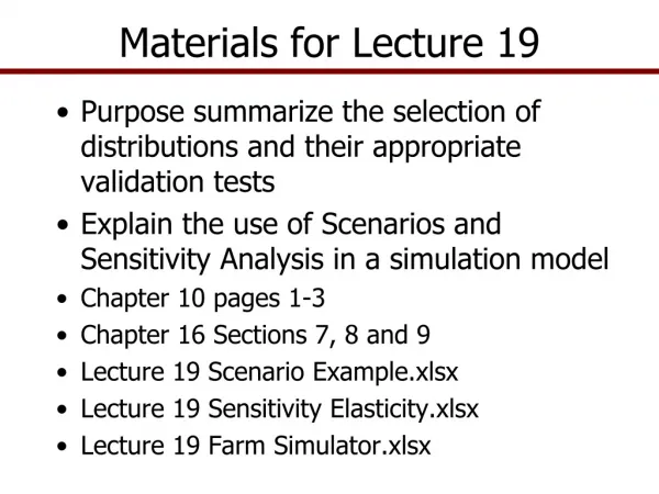
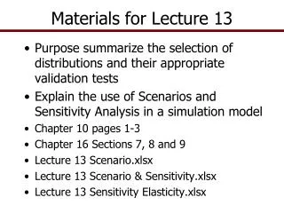
Materials for Lecture 13 • Purpose summarize the selection of distributions and their appropriate validation tests • Explain the use of Scenarios and Sensitivity Analysis in a simulation model • Chapter 10 pages 1-3 • Chapter 16 Sections 7, 8 and 9 • Lecture 13 Scenario.xls • Lecture 13 Scenario & Sensitivity.xls • Lecture 13 Sensitivity Elasticity.xls
Summarize Validation Tests • Validation of simulated distributions is critical to building good simulation models • Selection of the appropriate statistical tests to validate the simulated random variables is essential • Appropriate statistical tests changes as we change the method for estimating the parameters
Summarize Univariate Validation Tests • If the data are stationary and you want to simulate using the historical mean • Distribution • Use Normal as =NORM(Ῡ, σY) or • Empirical as =EMP(Historical Ys) • Validation Tests for Univariate distribution • Compare Two Series tab in Simetar • Student-t test of means as H0: ῩHist = ῩSim • F test of variances as H0: σ2Hist = σ2Sim • You want both tests to Fail to Reject the null H0
Summarize Univariate Validation Tests • If the data are stationary and you want to simulate using a mean that is not equal to the historical mean • Distribution • Use Empirical as a fraction of the mean so the Si = Sorted((Yi - Ῡ)/Ῡ) and simulate using the formula Ỹ = Ῡ(new mean) * ( 1 + EMP(Si, F(Si), [CUSDi] )) • Validation Tests for Univariate distribution • Test Parameters • Student-t test of means as H0: ῩNew Mean = ῩSim • Chi-Square test of Std Dev as H0: σHist = σSim • You want both tests to Fail to Reject the null H0
Summarize Univariate Validation Tests • If the data are non-stationary and you use OLS, Trend, or time series to project Ŷ • Distribution • Use =NORM(Ŷ , Standard Deviation of Residuals) • Use Empirical and the residuals as fractions of Ŷ calculated for Si = Sorted((Yi - Ŷj)/Ŷ) and simulate each variable using Ỹi = Ŷi * (1+ EMP(Si, F(Si) )) • Validation Tests for Univariate distribution • Test Parameters • Student-t test of means as H0: ŶNew Mean = ῩSim • Chi-Square test of Std Dev as H0: σê = σSim • You want both tests to Fail to Reject the null H0
Summarize Univariate Validation Tests • If the data have a cycle, seasonal, or structural pattern and you use OLS or any econometric forecasting method to project Ŷ • Distribution • Use =NORM(Ŷ, σê standard deviation of residuals) • Use Empirical and the residuals as fractions of Ŷ calculated for Si = Sorted((Yi - Ŷ)/Ŷ) and simulate using the formula Ỹ = Ŷ * (1 + EMP(Si, F(Si) )) • Validation Tests for Univariate distribution • Test Parameters tab • Student-t test of means as H0: ŶNew Mean = ῩSim • Chi-Square test of Std Dev as H0: σê = σSim • You want both tests to Fail to Reject the null H0
Summarize Multivariate Validation Tests • If the data are stationary and you want to simulate using the historical means and variance • Distribution • Use Normal =MVNORM(Ῡ vector, ∑ matrix) or • Empirical =MVEMP(Historical Ys,,,, Ῡ vector, 0) • Validation Tests for Multivariate distributions • Compare Two Series for 10 or fewer variables • Hotelling T2 test of mean vectors as H0: ῩHist = ῩSim • Box’s M Test of Covariances as H0: ∑Hist = ∑Sim • Complete Homogeneity Test of mean vectors and covariance simultaneously • You want all three tests to Fail to Reject the null H0 • Check Correlation • Performs a Student-t test on each correlation coefficient in the correlation matrix: H0: ρHist = ρSim • You want all calculated t statistics to be less than the Critical Value t statistic so you fail to reject each t test (Not Bold)
Summarize Multivariate Validation Tests • If you want to simulate using projected means such that Ŷt ≠ Ῡhistory • Distribution • Use Normal as = MVNORM(Ŷ Vector, ∑matrix) or • Empirical as = MVEMP(Historical Ys ,,,, Ŷ vector, 2) • Validation Tests for Multivariate distribution • Check Correlation • Performs a Student-t test on each correlation coefficient in the matrix: H0: ρHist = ρSim • You want all calculated t statistics to be less than the Critical Value t statistic so you fail to reject each t test • Test Parameters, for each j variable • Student-t test of means as H0: ŶProjected j = ῩSim j • Chi-Square test of Std Dev as H0: σê j = σSim j
Using a Simulation Model • Now lets change gears • Assume we have a working simulation model • The Model has the following parts • Input section where the user enters all input values that are management control variables and exogenous policy or time series data • Stochastic variables that have been validated • Equations to calculate all dependent variables • Equations to calculate the KOVs • A KOV table to send to the simulation engine
Scenario and Sensitivity Analysis • Simetar simulation engine controls • Number of scenarios • Sensitivity analysis • Sensitivity elasticities
Scenario loop IS = 1, M Change management variables (X) from one scenario to the next Iteration loop IT = 1, N Next scenario Scenario Analysis • Base scenario – complete simulation of the model for 500 or more iterations with all variables set at their initial or base values • Alternative scenario – complete simulation of the model for 500 or more iterations with one or more of the control variables changed from the Base • All scenarios must use the same random values Use the same random values for all random variables, so identical risk for each scenario
Scenario Analysis • All values in the model are held constant and you systematically change one or more variables • Number of scenarios determined by analyst • Random number seed is held constant and this forces Simetar to use the same random values for the stochastic variables for every scenario (Pseudo Random Numbers) • Use =SCENARIO() Simetar function to increment each of the scenario (manager) control variables
Example of a Scenario Table • 5 Scenarios for the risk and VC • Purpose is to look at the impacts of different management scenarios on net returns
Scenario Table of the Controls • Create as big of scenario table as needed • Add all control variables into the table
Sensitivity Analysis • Sensitivity analysis seeks to determine how sensitive the KOVs are to small changes in one particular variable • Does net return change a little or a lot when you change variable cost per unit? • Does NPV change greatly if the assumed fixed cost changes? • Simulate the model numerous times changing the “change” variable for each simulation • Must ensure that the same random values are used for each simulation • Simetar has a sensitivity option that insures the same random values used for each run
Sensitivity Analysis • Simetar uses the Simulation Engine to specify the change variable and the percentage changes to test • Specify as many KOVs as you want • Specify ONE sensitivity variable • Simulate the model and 7 scenarios are run
Demonstrate Sensitivity Simulation • Change the Price per unit as follows • + or – 5% • + or – 10% • + or – 15% • Simulates the model 7 times • The initial value you typed in • Two runs for + and – 5% for the control variable • Two runs for + and – 10% for the control variable • Two runs for + and – 15% for the control variable • Collect the statistics for only a few KOVs • For demonstration purposes collect results for the variable doing the sensitivity test on • Could collect the results for several KOVs
Sensitivity Results • Test Sensitivity of the price received for the product being manufactured on Net Cash Income
Sensitivity Elasticities (SE) • Sensitivity of a KOV with respect to (wrt) multiple variables in the model can be estimated and displayed in terms of elasticities, calculated as: SEij = % Change KOVi % Change Variablej • Calculate SE’s for a KOVi wrt change variablesj at each iteration and then calculate the average and standard deviation of the SE • SEij’s can be calculated for small changes in Control Variablesj, say, 1% to 5% • Necessary to simulate base with all values set initially • Simulate model for an x% change in Vj • Simulate model for an x% change in Vj+1
Sensitivity Elasticities • The more sensitive the KOV is to a variable, Vj, the larger the SEij • Display the SEij’s in a table and chart

