Materials for Lecture 13
Materials for Lecture 13. Purpose summarize the selection of distributions and their appropriate validation tests Explain the use of Scenarios and Sensitivity Analysis in a simulation model Chapter 10 pages 1-3 Chapter 16 Sections 7, 8 and 9 Lecture 13 Scenario.xls

Materials for Lecture 13
E N D
Presentation Transcript
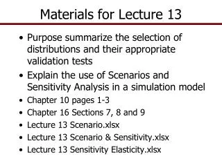
Materials for Lecture 13 • Purpose summarize the selection of distributions and their appropriate validation tests • Explain the use of Scenarios and Sensitivity Analysis in a simulation model • Chapter 10 pages 1-3 • Chapter 16 Sections 7, 8 and 9 • Lecture 13 Scenario.xls • Lecture 13 Scenario & Sensitivity.xls • Lecture 13 Sensitivity Elasticity.xls
Summarize Validation Tests • Validation of simulated distributions is critical to building good simulation models • Selection of the appropriate statistical tests to validate the simulated random variables is essential • The appropriate statistical test changes as we change the method for estimating the parameters
Summarize Univariate Validation Tests • If the data are stationary and you want to simulate using the historical mean • Distribution • Use Normal as =NORM(Ῡ, σY) or • Empirical as =EMP(Historical Ys) • Validation Tests for Univariate distribution • Compare Two Series tab in Simetar • Student-t test of means as H0: ῩHist = ῩSim • F test of variances as H0: σ2Hist = σ2Sim • You want both tests to Fail to Reject the null H0
Summarize Univariate Validation Tests • If the data are stationary and you want to simulate using a mean that is not equal tothe historical mean • Distribution • Use Empirical as a fraction of the mean so the Si = Sorted((Yi - Ῡ)/Ῡ) and simulate using the formula Ỹ = Ῡ(new mean) * ( 1 + EMP(Si, F(Si), [CUSDi] )) • Validation Tests for Univariate distribution • Test Parameters • Student-t test of means as H0: ῩNew Mean = ῩSim • Chi-Square test of Std Dev as H0: σHist = σSim • You want both tests to Fail to Reject the null H0
Summarize Univariate Validation Tests • If the data are non-stationaryand you use OLS, Trend, or time series to project Ŷ • Distribution • Use =NORM(Ŷ , Standard Deviation of Residuals) • Use Empirical and the residuals as fractions of Ŷ calculated for Si = Sorted((Yi - Ŷj)/Ŷ) and simulate each variable using Ỹi = Ŷi * (1+ EMP(Si, F(Si) )) • Validation Tests for Univariate distribution • Test Parameters • Student-t test of means as H0: ŶNew Mean = ῩSim • Chi-Square test of Std Dev as H0: σê = σSim • You want both tests to Fail to Reject the null H0
Summarize Univariate Validation Tests • If the data have a cycle, seasonal, or structural pattern and you use OLS or any econometric forecasting method to project Ŷ • Distribution • Use =NORM(Ŷ, σê standard deviation of residuals) • Use Empirical and the residuals as fractions of Ŷ calculated for Si = Sorted((Yi - Ŷ)/Ŷ) and simulate using the formula Ỹ = Ŷ * (1 + EMP(Si, F(Si) )) • Validation Tests for Univariate distribution • Test Parameters tab • Student-t test of means as H0: ŶNew Mean = ῩSim • Chi-Square test of Std Dev as H0: σê = σSim • You want both tests to Fail to Reject the null H0
Summarize Multivariate Validation Tests • If the data are stationary and you want to simulate using the historical means and variance • Distribution • Use Normal =MVNORM(Ῡ vector, ∑ matrix) or • Empirical =MVEMP(Historical Ys,,,, Ῡ vector, 0) • Validation Tests for Multivariate distributions • Compare Two Series for 10 or fewer variables • Hotelling T2 test of mean vectors as H0: ῩHist = ῩSim • Box’s M Test of Covariances as H0: ∑Hist = ∑Sim • Complete Homogeneity Test of mean vectors and covariance simultaneously • You want all three tests to Fail to Reject the null H0 • Check Correlation • Performs a Student-t test on each correlation coefficient in the correlation matrix: H0: ρHist = ρSim • You want all calculated t statistics to be less than the Critical Value t statistic so you fail to reject each t test (Not Bold)
Summarize Multivariate Validation Tests • If you want to simulate using projected means such that Ŷt ≠ Ῡhistory • Distribution • Use Normal as = MVNORM(Ŷ Vector, ∑matrix) or • Empirical as = MVEMP(Historical Ys ,,,, Ŷ vector, 2) • Validation Tests for Multivariate distribution • Check Correlation • Performs a Student-t test on each correlation coefficient in the matrix: H0: ρHist = ρSim • You want all calculated t statistics to be less than the Critical Value t statistic so you fail to reject each t test • Test Parameters, for each j variable • Student-t test of means as H0: ŶProjected j = ῩSim j • Chi-Square test of Std Dev as H0: σê j = σSim j
Using a Simulation Model • Now lets change gears • Assume we have a working simulation model • The Model has the following parts • Input section where the user enters all input values that are management control variables and exogenous policy or time series data • Stochastic variables that have been validated • Equations to calculate all dependent variables • Equations to calculate the KOVs • A KOV table to send to the simulation engine
Scenario and Sensitivity Analysis • Simetar simulation engine controls • Number of scenarios • Sensitivity analysis • Sensitivity elasticities
Scenario loop IS = 1, M Change management variables (X) from one scenario to the next Iteration loop IT = 1, N Next scenario Scenario Analysis • Base scenario – complete simulation of the model for 500 or more iterations with all variables set at their initial or base values • Alternative scenario – complete simulation of the model for 500 or more iterations with one or more of the control variables changed from the Base • All scenarios must use the same random values Use the same random values for all random variables, so identical risk for each scenario
Scenario Analysis • All values in the model are held constant and you systematically change one or more variables • Number of scenarios determined by analyst • Random number seed is held constant and this forces Simetar to use the same random values for the stochastic variables for every scenario • Use =SCENARIO() Simetar function to increment each of the scenario control variables
Example of a Scenario Table • 5 Scenarios for the risk and VC • Purpose is to look at the impacts of different management scenarios on net returns
Scenario Table of the Controls • Create as big of table as needed • Add all control variables into the table
Sensitivity Analysis • Sensitivity analysis seeks to determine how sensitive the KOVs are to small changes in one particular variable • Does net return change a little or a lot when you change variable cost per unit? • Does NPV change greatly if the assumed fixed cost changes? • Simulate the model numerous times changing the “change” variable for each simulation • Must ensure that the same random values are used for each simulation • Simetar has a sensitivity option that insures the same random values used for each run
Sensitivity Analysis • Simetar uses the Simulation Engine to specify the change variable and the percentage changes to test • Specify as many KOVs as you want • Simulate the model and 7 scenarios are run
Demonstrate Sensitivity Simulation • Change the Price per unit as follows • + or – 5% • + or – 10% • + or – 15% • Simulates the model 7 times • The initial value you typed in • Two runs for + and – 5% for the control variable • Two runs for + and – 10% for the control variable • Two runs for + and – 15% for the control variable • Collect the statistics for only few KOVs • For demonstration purposes collect results for the variable doing the sensitivity test on • Could collect the results for several KOVs
Sensitivity Results • Test Sensitivity of the price received for the product being manufactured on Net Cash Income
Sensitivity Elasticities (SE) • Sensitivity of a KOV with respect to (wrt) multiple variables in the model can be estimated and displayed in terms of elasticities, calculated as: SEij = % Change KOVi % Change Variablej • Calculate SE’s for a KOVi wrt change variablesj at each iteration and then calculate the average and standard deviation of the SE • SEij’s can be calculated for small changes in Control Variablesj, say, 1% to 5% • Necessary to simulate base with all values set initially • Simulate model for an x% change in Vj • Simulate model for an x% change in Vj+1
Sensitivity Elasticities • The more sensitive the KOV is to a variable, Vj, the larger the SEij • Display the SEij’s in a table and chart


