Download
1 / 16
160 likes | 300 Views
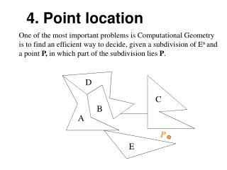
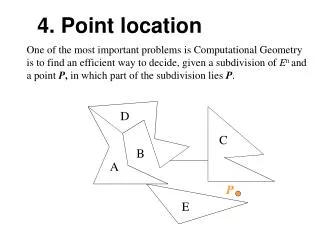
4. Point location. One of the most important problems is Computational Geometry is to find an efficient way to decide, given a subdivision of E n and a point P , in which part of the subdivision lies P. D. C. B. A. P. E. Point location (cont.).

E N D
4. Point location One of the most important problems is Computational Geometry is to find an efficient way to decide, given a subdivision of En and a point P, in which part of the subdivision lies P. D C B A P E
Point location (cont.) A natural way to start the search is to divide the plane into vertical stripes and to decide the position of P in two steps: - the stripe, (1) - the facet of the stripe(2). D C B A P E
Point location (cont.) But it turn out that the number of facets in this construction can be O (n2) in terms of the number of edges! Example with 2(1 + 2 + 3 +...+ n) + 1 + n = (n+1)2 facets! If the vertical lines end at the fist intersection with the edges of the subdivision, the number of trapezoids is N 3 n+ 1 (eq. 4.1).
Point location (cont.) D C B A R E In this counting and further, we assume that, unlike the vertices of C, no two vertices of the subdivision have equal y coordinates, i.e. we assume that the edges of the subdivision are in general position.
Point location (cont.) This subdivision has the property that each trapezoid has unique upper bounding edge top (), unique lower bounding edge bottom (), unique left vertex leftp (), and unique right vertex rightp (). Each trapezoid has also 1-2 left and 1-2 right neighbors, e.g. lln () is its left lower neighbor. top () leftp () Right upper neighbor rightp () bottom ()
Point location (cont.) Back to eq. 4.1. • The number of trapezoids is L + 1 where L is the number of the vertices leftp (), since each trapezoid, with the exception of the leftmost one, has exactly one such vertex. 1 2 • The left endpoint of a segment may be leftp () for at most 2 trapezoids, whereas the right one for at most 1 trapezoid. Therefore n initial segments define at most 3n trapezoids, which proves eq. 4.1. It is easy to see that there are no more than 6n + 4 vertices (4 vertices of the rectangle R included).
Point location (Trapezoidal Map) Algorithm 8 = Trapezoidal Map The algorithm is incremental on the set of edges. So we may think about the structure as about a set S of edges. Adding edge at a time we update the data structure and the search structure. Theedges may have only endpoints in common. They are not sorted. (1) Data structure (DS): For each facet we save: - leftp (), rightp (), top (), bottom (), and its neighbors.
Point location (Trapezoidal Map) • (2) Search Structure (SS): Oriented graph without loops, whose • - leafs are trapezoids of the Trapezoidal Map, • inner nodes are the edges from the initial set S, or their • endpoints. • There is exactly one root. The out degree of inner nodes is 2. • If the inner node is an edge the deciding criterion is above or • below*, if this is a point the criterion is left of right. • DS and SS are used not only to finally locate the given point, but also to build DS and SS inductively! More precisely, • in the step i we first locate the endpoints of the edge si wrt already • constructed SSi-1 after the step i-1, • then we again use DSi-1 to determine the trapezoids • intersected by si. • *above will be depicted as „left“, below as „right“
s1 B q1 E D Example1. p1 p2 s2 C G A F q2 F1 F2 p1 q1 q2 s1 A G s2 B E p2 C U F1U D s2 F C E U F2U G D
s1 B q1 E q3 D Example2. p1 G p2 s3 H C I A F s2 q2 = p3 p1 q1 q2 s1 A q3 s2 B H s3 E p2 s2 C F I G D
Example3. A q i B 0 s i D C pi pi q i 0 s i A D C B
Example4.1 2 q i C2 1 B2 D2 s i A2 q i 3 D1 E C1 s i pi B1 pi 0 A1 q i F The glueing process is necessary because the vertical lines intersected with si need to be shortend to the first intersection! B D s i E C pi A
Example4.2 s i s i s i q i E 0 1 2 3 A1 A2 B1 B2 C1 C2 s i B2 s i D1 D2 B1 s i s i s i q i E q i A F s i D2 s i C D1 E B D
Point location (Trapezoidal Map, expected behavior) Theorem. A planar subdivision with n edges in general position admits an algorithm (1) whose running timehas expected O (n log n) time, (2) the storage requires O (n) time, and (3) the location of a given point q takes expected O (log n) time. Proof of (2): - At each step i kileafs (trapezoids) and (k i - 1) inner nodes (easy to check) are produced. E(ki) =number of leafs * probability a leaf is obtained in the step I =O(i) * 4/I = O(1)
Point location (Trapezoidal Map, expected behavior) Proof of (3): Let Xi be the number of nodes on the search path to q constructed in step i (in Example 1 (the path to q)X1=X2=3), and letE(X) be the expected value of X. Then: p1 X1 q1 s1 p2 X2 s2 F s1 B q1 E D p1 p2 C G s2 q A q2 F • - In the step i the path leading to q is increased by at most 3 nodes. • - The increase happens only when a trapezoid of q is changed. • The change may only happen if si is top (), bottom (), or defines • leftp () or rightp (), where is the new trapezoid! of q.
Point location (Trapezoidal Map, expected behavior) • Proof of (3) – cont.: • The probability of each of these events is 1/i • total = 3•4• 1/i. • Now E(X i) = 12/i = O (log n). Proof of (1): - O (log i) needed to locate the left endpoint of e i - O (ki) needed for the nodes in SSi produced by e i Hence, (O (log i) + O (E (ki)) ) = O (n log n) + O (n) = O (n log n)