Download
1 / 55
550 likes | 575 Views
Explore the usefulness of MODIS SST as an Essential Climate Variable, its application in NWP and oceanography, and techniques for measuring and validating SST data. Learn about the uncertainties in Satellite-derived CDRs and the spatial distribution of errors in SST measurements.

E N D
Sea-Surface Temperature from MODIS Peter J Minnett, Robert H Evans and Gui Podestá Meteorology and Physical Oceanography Rosenstiel School of Marine and Atmospheric ScienceUniversity of Miami
Overview • Sea-surface temperature (SST) as an Essential Climate Variable (ECV), and Climate Data Record (CDR) • MODIS SSTs • Improvements in the atmospheric correction algorithms • Radiometric measurements of SSTs from ships • Traceability to SI standards • Physical processes at the sea surface • Diurnal heating and cooling • Thermal skin effect
Sea-surface temperature • Temperature is a fundamental SI variable. • SST is an important variable, helps determine the coupling between ocean and atmosphere. • Has many applications in NWP, operational oceanography, climate studies. • Can be measured to good accuracy from space. • Can be validated to determine residual uncertainties.
Satellite-derived CDRs • National Academy of Sciences Report (NRC, 2000): “a data set designed to enable study and assessment of long-term climate change, with ‘long-term’ meaning year-to-year and decade-to-decade change. Climate research often involves the detection of small changes against a background of intense, short-term variations.” • “Calibration and validation should be considered as a process that encompasses the entire system, from the sensor performance to the derivation of the data products. The process can be considered to consist of five steps: • instrument characterization, • sensor calibration, • calibration verification, • data quality assessment, and • data product validation.”
Desired SST CDR uncertainties • The useful application of all satellite-derived variables depends on a confident determination of uncertainties. • CDRs of SSTs require most stringent knowledge of the uncertainties: • Target accuracies: 0.1K over large areas, stability 0.04K/decade - Ohring et al. (2005) Satellite Instrument Calibration for Measuring Global Climate Change: Report of a Workshop. Bulletin of the American Meteorological Society 86:1303-1313
What is SST? • The infrared emission from the ocean originates from the uppermost <1mm of the ocean – the skin layer. • The atmosphere is in contact with the top of the skin layer. • Ocean-to-atmosphere heat flow through the skin layer is by molecular conduction: this causes, and results from, a temperature gradient through the skin layer. • Conventional measurements of SST are from submerged thermometers – a “bulk” temperature. • Tdepth below the influence of diurnal heating is the “foundation” temperature. From Eifler, W. and C. J. Donlon, 2001: Modeling the thermal surface signature of breaking waves. J. Geophys. Res., 106, 27,163-27,185.
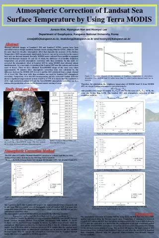
The SST atmospheric correction algorithms The form of the daytime and night-time algorithm for measurements in the long wave atmospheric window is: SST = c1 + c2 * T11 + c3 * (T11-T12) * Tsfc+ c4 * (sec (θ) -1) * (T11-T12) where Tn are brightness temperatures measured in the channels at nm wavelength, Tsfc is a ‘climatological’ estimate of the SST in the area, and θ is the satellite zenith angle. This is based on the Non-Linear SST algorithm. [Walton, C. C., W. G. Pichel, J. F. Sapper and D. A. May (1998). "The development and operational application of nonlinear algorithms for the measurement of sea surface temperatures with the NOAA polar-orbiting environmental satellites." Journal of Geophysical Research103 27,999-28,012.] The MODIS night-time algorithm, using two bands in the 4m atmospheric window is: SST4= c1 + c2 * T3.9 + c3 * (T3.9-T4.0) + c4 * (sec (θ) - 1) Note, the coefficients in each expression are different. They can be derived in three ways: • empirically by regression against SST values derived from another validated satellite instrument • empirically by regression against SST values derived surface measurements from ships and buoys • theoretically by numerical simulations of the infrared radiative transfer through the atmosphere.
Uncertainty estimates Each processing step is prone to additional error sources. From Cornillon et al, 2010, Sea-Surface Temperature Error Budget White Paper. (http://www.ssterrorbudget.org/ISSTST/)
Uncertainty estimates Each processing step is prone to additional error sources. From Cornillon et al, 2010, Sea-Surface Temperature Error Budget White Paper. (http://www.ssterrorbudget.org/ISSTST/)
Spatial distribution of errors Areas of high bias errors can be related to geophysical phenomena: aerosols, upwelling, diurnal heating, anomalous humidity distributions ….
Where next? • Refine NLSST with regionally as well as seasonally optimized coefficient sets – “Latband algorithm” • Use advanced computational techniques: • Genetic Algorithm (GA)-based equation discovery to derive alternative forms of the correction algorithm • Regression tree to identify geographic regions with related characteristics • Support Vector Machines (SVM) to minimize error using state-of-the-art non-linear regression
“Latband” improvements Time series of mean SST residuals for MODIS-Aqua. Algorithm coefficients estimated for six fixed latitudinal bands and for each month of the year. V6 – with “LATBAND” approach. V5 – without. Version 6 Version 5
Equation Discovery using Genetic Algorithms • Darwinian principles are applied to algorithms that “mutate” between successive generations • The algorithms are applied to large data bases of related physical variables to find robust relationships between them. Only the “fittest” algorithms survive to influence the next generation of algorithms. • Here we apply the technique to the MODIS matchup-data bases. • The survival criterion is the size of the RMSE of the SST retrievals when compared to buoy data.
Genetic Mutation of Equations • The initial populationof formulae is created by a generator of random algebraic expressions from a predefined set of variables and operators. For example, the following operators can be used: {+, -, /, ×, √, exp, cos, sin, log}. To the random formulae thus obtained, we can include “seeds” based on published formulae, such as those already in use. • In the recombination step, the system randomly selects two parent formulae, chooses a random subtree in each of them, and swaps these subtrees. • The mutation of variablesintroduces the opportunity to introduce different variables into the formula. In the tree that defines a formula, the variable in a randomly selected leaf is replaced with another variable.
Successive generations of algorithms The formulae are represented by tree structures; the “recombination” operator exchanges random subtrees in the parents. Here the parent formulae (yx+z)/log(z) and (x+sin(y))/zy give rise to children formulae (sin(y)+z)/log(z) and (x+yx)/zy. The affected subtrees are indicated by dashed lines. Subsets of the data set can be defined in any of the available parameter spaces. (From Wickramaratna, K., M. Kubat, and P. Minnett, 2008: Discovering numeric laws, a case study: CO2 fugacity in the ocean. Intelligent Data Analysis, 12, 379-391.)
And the winner is…. The “fittest” algorithm takes the form: where: Ti is the brightness temperature at λ= iµm θsis the satellite zenith angle θais the angle on the mirror (a feature of the MODIS paddle-wheel mirror design) Which looks similar to the NLSST:
MODIS scan mirror effects Mirror effects: two-sided paddle wheel has a multi-layer coating that renders the reflectivity in the infrared a function of wavelength, angle of incidence and mirror side.
Variants of the new algorithms Coefficients are different for each equation Note: No Tsfc
Regression tree • Regions identified by the regression tree algorithm • The tree is constructed using • input variables: latitude and longitude • output variable: Error in retrieved SST • Algorithm recursively splits regions to minimize variance within them • The obtained tree is pruned to the smallest tree within one standard error of the minimum-cost subtree, provided a declared minimum number of points is exceeded in each region • Linear regression is applied separately to each resulting region (different coefficients result)
Regression tree performance • Terra 2004 SSTday NLSST (no regions) – RMSE: 0.581 New formula (no regions) – RMSE: 0.615 New formula (with regions) – RMSE: 0.568 • Terra 2004 SST4 (night) SST4 (no regions) – RMSE: 0.528 New formula (no regions) – RMSE: 0.480 New formula (with regions) – RMSE: 0.456
Support Vector Machines (SVM) • Best accuracy observed when data set is large (lower accuracy when splitting into regions) • Terra 2004 SSTday– • RMSE (no region): 0.513, RMSE (with regions): 0.557 • Problems: • Computational costs • Black-box approach
Preliminary Results • The new algorithms with regions give smaller errors than NLSST or SST4 • Tsfc term no longer required • Night-time 4µm SSTs give smallest errors • Aqua SSTs are more accurate than Terra SSTs • Regression-tree induced in one year can be applied to other years without major increase in uncertainties • SVM results do not out-perform GA+Regression Tree algorithms
Next steps • Can some regions be merged without unacceptable increase in uncertainties? • 180oW should not necessarily always be a boundary of all adjacent regions. • Iterate back to GA for regions – different formulations may be more appropriate in different regions. • Allow scan-angle term to vary with different channel sets. • Introduce “regions” that are not simply geographical.
Validation and CDR generation • Validation required over life-time of mission • Should encompass all atmospheric and oceanic variability. • Traceability to SI standards is needed. → ship-based radiometers
Marine-Atmospheric Emitted Radiance Interferometer The M-AERI is a Michelson-Morley Fourier-transform infrared interferometricspectroradiometer. These were first developed in the 1880’s to make accurate measurements of the speed of light. Here we use it to make very accurate measurements of the sea-surface temperature, air temperature and profiles of atmospheric temperature and humidity. We also measure surface emissivity and the temperature profile through the skin layer, which is related to the flow of heat from the ocean to the atmosphere.
Ocean and atmosphere infrared spectra NB: X10 change in temperature scale Examples of parts of spectra measured by the M-AERI, represented as temperature, and those intervals where the sky temperatures are smallest indicate where the atmosphere is most transparent. The spikes in the atmospheric spectra are caused by emission lines. The blue bar shows which spectral region is used to measure air temperature, and the red bar skin sea-surface temperature. Note the change in temperature scales of the two panels. These data were taken in the Tropical Western Pacific during the Combined Sensor Program Cruise in 1996. From Minnett, P. J., R. O. Knuteson, F. A. Best, B. J. Osborne, J. A. Hanafin and O. B. Brown (2001). "The Marine-Atmospheric Emitted Radiance Interferometer (M-AERI), a high-accuracy, sea-going infrared spectroradiometer." Journal of Atmospheric and Oceanic Technology. 18(6): 994-1013.
M-AERI cruises for MODIS, AATSR & AVHRR validation Explorer of the Seas Explorer of the Seas: near continuous operation December 2000 – December 2007. Restarted February 2010.
Measuring skin SST from ships • Scan-mirror mechanism for directing the field of view at complementary angles. • Excellent calibration for ambient temperature radiances. • Moderately good calibration at low radiances.
Sea surface emissivity (ɛ) Conventional wisdom gave decreasing ε with increasing wind. Not confirmed by at-sea hyperspectral measurements Improved modeling confirms at-sea measurements. Hanafin, J. A. and P. J. Minnett, 2005: Infrared-emissivity measurements of a wind-roughened sea surface. Applied Optics., 44, 398-411. Nalli, N. R., P. J. Minnett, and P. van Delst, 2008: Emissivity and reflection model for calculating unpolarized isotropic water surface-leaving radiance in the infrared. I: Theoretical development and calculations. Applied Optics, 47, 3701-3721. Nalli, N. R., P. J. Minnett, E. Maddy, W. W. McMillan, and M. D. Goldberg, 2008: Emissivity and reflection model for calculating unpolarized isotropic water surface-leaving radiance in the infrared. 2: Validation using Fourier transform spectrometers. Applied Optics, 47, 4649-4671.
NIST water-bath black-body calibration target See: Fowler, J. B., 1995. A third generation water bath based blackbody source, J. Res. Natl. Inst. Stand. Technol., 100, 591-599
CDR of SST Satellite-derived SSTs NIST Traceable error statistics M-AERI, ISAR…. measurements Matchup analysis of collocated measurements Laboratory calibration NIST-designed water-bath blackbody calibrator NIST-traceable thermometers NIST TXR for radiometric characterization
Next-generation ship-based FTIR spectroradiometer M-AERI Mk-2 undergoing tests at RSMAS.
Skin – bulk SST differences Example of wind speed dependence of diurnal & skin effects – off Baja California From: Minnett, P. J., 2003: Radiometric measurements of the sea-surface skin temperature - the competing roles of the diurnal thermocline and the cool skin. International Journal of Remote Sensing, 24, 5033-5047.
Skin effect • Caused by molecular conduction being the mechanism for heat flow from ocean to atmosphere. • First order correction: ΔT ≈ 0.2K • Better correction requires: • accurate wind-speeds for U10<7ms-1, • net infrared heat flux at the surface, • incident solar radiation at the surface, • SST. σ= ±0.095K. From: Minnett, P. J., M. Smith and B. Ward (2011). Measurements of the oceanic thermal skin effect. Deep Sea Research II. In the press.