Sea Surface
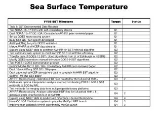
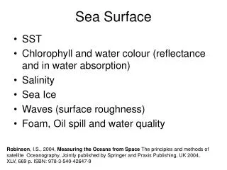
Sea Surface. SST Chlorophyll and water colour (reflectance and in water absorption) Salinity Sea Ice Waves (surface roughness) Foam, Oil spill and water quality.

Sea Surface
E N D
Presentation Transcript
Sea Surface • SST • Chlorophyll and water colour (reflectance and in water absorption) • Salinity • Sea Ice • Waves (surface roughness) • Foam, Oil spill and water quality Robinson, I.S.,2004, Measuring the Oceans from Space The principles and methods of satellite Oceanography. Jointly published by Springer and Praxis Publishing, UK 2004, XLV, 669 p. ISBN: 978-3-540-42647-9
T10 T12 Sea Surface Temperature DRY MOIST T10-T12 [K] SST= a*T10+b*(T10-T12)+c
Comments on applications for air-sea interaction • SST is needed for estimation of LWup component of the radiation budget, as well as to estimate the saturation humidity for latent heat flux, in the estimation of sensible heat flux and of the evaporation. • Study of evolution of SST fields may be of interest in process description.
Data characteristics • Spatial resolution ranges from medium (1-10 km from every 12hours to 15’ e large (10-100 km) (interferometers, MW radiometers) • Archived data >25 years (e.g. Pathfinder) • Current best (potential) Temporal resolution: 15’ for about 5x5km data. • MW based products are available at relatively low resolutions (>10 km) and only over open oceans. • Accuracy 0.5 K (IR & cloud free)
Weaknesses • Skin vs bulk temperature • Lack of large datasets for diurnal cycle studies • Problems with coasts, undetected clouds (for IR based) and aerosol contamination. • Assumptions on the air temperature vertical structure. • Clouds (IR based)
Ocean Colour Satellite measurement of ocean colour consists in dedicated* spectral measurements of visible radiation with channels that corresponds to the actual colours. *the instrument must be optimized in the range of low values of reflectivity (SPOT, Landsat are not optimized) Source: http://cimss.ssec.wisc.edu/satmet/home/poes_florida.html
Ocean color depends from • Pure seawater optical characteristics • Phytoplankton • DOM (Dissolved Organic Material) or Yellow substance or gelbstoff • Suspended particular matter • Seafloor color (shallow waters) • Foam • Oil spills • Sunglint
Applications of ocean colour derived parameters • Diffuse attenuation coefficient (Kλ): physical modeling -> thermal structure biological modeling -> available underwater solar radiation characterization of ocean waters • Phytoplankton biomass biological modeling -> primary production (CO2 fluxes) • Water quality parameters • Seabed characterization • Tracer for dynamic processes
Data characteristics • Spatial resolution is about 1 km. • Temporal sampling: For a single low orbit satellite in principle it is possible to have a measurement each 24 hours. Gaps in the swaths, clouds, aerosols and sunglint reduce the effective temporal sampling. • Archived data about 10 years (e.g. SeaWifs) from the same platform. Archived observations are available since 1978 (CZCS) but there have been no missions for about 10 years (1986-96)
Weaknesses • Clouds and aerosols and in general atmospheric contribution. • Problems (seabed, land contamination, sediments etc..) in coastal areas for phytoplankton estimation • Need for regional algorithms • Assumptions on the effective vertical structure of phytoplankton for CO2 fluxes estimation.
Stima della clorofilla tramite ‘ocean colour’ Rapporto BLU/VERDE Relationship between in situ chlorophyll concentration and the Remote Sensing Reflectances band ratios. Red crosses are the data used in the algorithms development. Blue crosses are the new data collected in the Mediterranean. Lines indicate the remote sensing algorithms (OC2-V4 dotted line, NL-DORMA solid line)
Ls=Lp+Lr+Lw Lp=F(aerosols,p) Lr=F(observation geometry, wind (foam, roughness, glint)) Aerosols=F(Ls670,Ls870)
205 153 52 0 153 52 21 235 108 255 235 108
Why should we measure SSS? • Key oceanographic (density) and climatic parameter • Thermohaline circulation / heat fluxes • Variations due to E-P budget, freezing/melting, freshwater run-off • 24% NEVER sampled and 40% less than 5 samples • Oceanographicmodels already assimilate SST and SSH from satellite data, while SSS is still climatologic Conveyor Belt SSS time-series • Prospective benefits: • Thermohaline circulation monitoring • Ocean precipitation rate estimates • Barrier layer effect • Annual/inter-annual variability (ENSO)
1.4 GHz, L-band (dedicated) • Optimum SSS sensitivity • Reasonable pixel dimension • Atmosphere almost transparent Configuration Parameters (f, p, θ, φ) Scene Parameters (SSS,SST, sea state)
Motivation/OverviewWhat will we measure? Correction terms to be applied in TB computation Cosmic and galactic radiation Faraday effect Atmospheric contributions and losses Observed scene
Uncertainty in SMOS salinity measurement Instrumental errors • Radiometric sensitivity, accuracy, calibration stability • Uncomplete characterisation of the system elements • Interferometric image reconstruction Geophysical effects to be accounted for • Ionosphere (Faraday rotation) • Atmosphere (dry air absorption, water vapour, clouds, rain) • External radiation (galactic background, sun, moon reflexions) • Sea surface temperature • Surface roughness (wind waves, swell, foam) Radio frequency interference
Chen, H.S., 1985. Space Remote Sensing Systems: An introduction. Academic Press. 258 pp.
SMOS • Sun-synchronous orbit • h=755 Km (LEO) • 3 days revisit time • Launch: October 31st, 2008 • 69 elements array, 120º spaced • d= 0.875 λ (Nyquist criterion unaccomplished) • Dual-pol / Full-pol • Multi-angular capabilities • Free-alias FOV about 1000 Km: no phase difference ambiguity • Spatial Reisolution: 35 Km (boresight)
Motivation/OverviewHow should we measure SSS? MIRAS(Microwave Imaging Radiometer by Aperture Synthesis) Complex cross-correlations between each antenna pair signals generate Visibility points u v
SSS Retrieval Cost function • Levenberg-Marquardt method • Multi-parameter (SSS, SST, U10) retrieval • Fixed upper and lower boundaries • Semi-empirical TB forward model • A priori knowledge of the auxiliary data errors • Mean sea level slope rather than wind
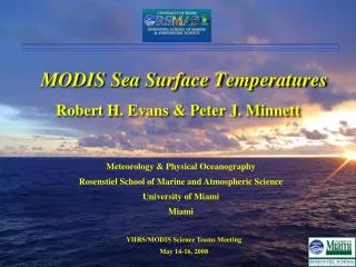
Salinity • Salinity can be retrieved with passive MW radiometry based on the fact that a change in salinity would introduce a change in the dielectric properties (emissivity) of sea water in the MW. • Retrieval of salinity requires the knowledge of SST, as well as the knowledge of atmospheric properties and other sea surface factors that are reponsible for the value of emissivity (e.g. wind) • Although attempt to retrieve salinity has been done with 6.6 Ghz (SMMR) lower frequencies (1-2 GHz) are needed • 2 satellites should be launched shortly for such mission (SMOS (ESA) and Aquarius (NASA+ Argentina's Comisión Nacional de Actividades Espaciales) • Spatial resolution will be quite coarse > 10 km and problem close to the coast
Starting in 2009, Aquarius mission will measure global SSS with unprecedented resolution. The science instruments will include a set of three radiometers that are sensitive to salinity (1.413 GHz; L-band) and a scatterometer that corrects for the ocean's surface roughness. The spacecraft will be contributed by Argentina's Comisión Nacional de Actividades Espaciales (CONAE).
Ice • Sea ice can be retrieved MW radiometry based on the fact that being of fresh water it will have different dielectric properties (emissivity) compared to sea water • Spatial resolution will be quite coarse > 10 km and problem close to the coast • Active MW sensing
Oil spill Due to the nature of an oil slick a satellite remote sensing platform is required to have the following: • High temporal resolution, due to the changing nature of the oil and its immediate threat to ecosystem, • The ability to image a given area regardless of cloud cover and prevailing weather conditions (even time of day), • High spatial resolution, to identify individual small oil patches (windrows), • Wide spectral resolution, as the position and width of the spectral band is important in distinguishing the oil from the adjacent water (Clark, 1993). • http://cearac.poi.dvo.ru/en/background/techniques/
OIL SPILL: VIS Crude and heavy refined oils have 3 optical properties which vary slightly from oil to oil, and which make them detectable at sea by optical sensors: • Their refractive index is greater than that of seawater • Their coefficient of light absorption is much stronger than that of water, particularly at shorter wavelengths • They fluoresce when subjected to bright natural light
Surface emissivity - Oceans Plane surface: Sea-water permittivity Fresnel equations (I, Q) Wind roughened surface: Sea-water permittivity Fresnel equations (I, Q) Large-scale waves Gravity-capillary, capillary waves (> 2m/s) RTTOV FASTEM-2 Whitecaps (> 7 m/s) Foam (> 10-12 m/s) Directional wind roughened surface: Sea-water permittivity Fresnel equations (I, Q, U, V) Large-scale waves Gravity-capillary, capillary waves (> 2m/s) RTTOV FASTEM-3 Whitecaps (> 7 m/s) Foam (> 10-12 m/s)
Sensitivity of surface emission (EoTs) to real and imaginary part of dielectric constant (Meissner and Wentz 2004) Modelled emissivity - Oceans 10.7 GHz 19.35 GHz = 53.1o = 0, 180o v-pol. h-pol. 37.0 GHz 85.5 GHz Wind speed [m/s]
3rd Stokes Vector at 10.7 GHz: Models vs. Windsat Data Data Coppo et al. (1996) Liu and Weng (2002) Wind speed < 4 m/s Windspeed: 4-8 m/s Relative azimuth angle [deg.] Relative azimuth angle [deg.] Windspeed: 8-12 m/s Windspeed > 12 m/s Relative azimuth angle [deg.] Relative azimuth angle [deg.] Stephen English Met Office
4th Stokes Vector at 19.35 GHz: Models vs. Windsat Data Liu and Weng (2002) Coppo et al. (1996) Data Wind speed < 4 m/s Windspeed: 4-8 m/s Relative azimuth angle [deg.] Relative azimuth angle [deg.] Windspeed: 8-12 m/s Windspeed > 12 m/s Relative azimuth angle [deg.] Relative azimuth angle [deg.] Stephen English Met Office
Sun-glint Sufficient Data sample Ralf Bennartz University of Wisconsin