Download
1 / 1
10 likes | 126 Views
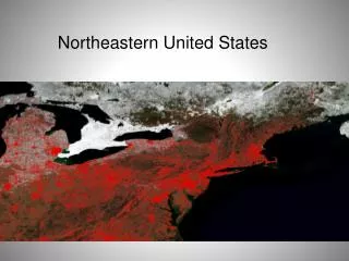
Synoptic and Mesoscale Aspects of Ice Storms in the Northeastern United States. A43C-0145. American Geophysical Union 2012 Fall Meeting San Francisco, CA 3 –7 December, 2012 Research supported by NOAA/CSTAR Grant: NA01NWS4680002.

E N D
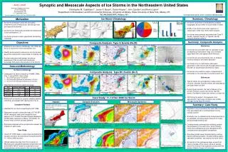
Synoptic and Mesoscale Aspects of Ice Storms in the Northeastern United States A43C-0145 American Geophysical Union 2012 Fall Meeting San Francisco, CA 3–7 December, 2012 Research supported by NOAA/CSTAR Grant: NA01NWS4680002 Christopher M. Castellano1*, Lance F. Bosart1, Daniel Keyser1, John Quinlan2, and Kevin Lipton2 1Department of Atmospheric and Environmental Sciences, University at Albany, State University of New York, Albany, NY 2NOAA/NWS/WFO Albany, NY *Corresponding author email: ccastellano@albany.edu Motivation Ice Storm Climatology Summary: Climatology N = 137 NTOT = 137 • Ice storms endanger human life and safety, undermine public infrastructure, and disrupt local and regional economies • Ice storms are historically prevalent and destructive in the northeastern U.S. • Ice storms present a major operational forecasting challenge • Ice storm occurrence is modulated by complex topography and proximity to large bodies of water • 81.8% of ice storms were local, regional, or subsynoptic, while only 18.2% were synoptic • Ice storms were primarily associated with Type G (N=65), Type BC (N=30), or Type EF (N=25) synoptic weather patterns NSYN = 25 Figure 1. Map indicating the 14 county warning areas (CWAs) included in the climatology. Figure 2. Archetypical surface synoptic weather patterns associated with freezing precipitation east of the Rocky Mountains. Caption and figure reproduced from Fig. 2 in Rauber et al. (2001). Figure 3. Number of ice storms impacting each county during the 1993–2010 period. Figure 4. Frequency distribution of ice storms by spatial coverage. Figure 5. Distribution of total ice storms (blue) and synoptic ice storms (red) by event type. Summary: Composite Analysis Objectives Composite Analysis: Type G Events (N=24) • Similarities • Ice storms are coincident with an upstream trough, an amplifying downstream ridge, and confluent upper-level flow over eastern North America • Ice storms are accompanied by low- to midlevel moisture transport and warm advection • Ice storms occur in association with quasi-geostrophic (QG) ascent and frontogeneticalforcing beneath an equatorward jet entrance region • Ice storms occur within a region of ageostrophic northerlies on the cold side of a surface warm font • Differences • Type G events are preceded by a deep cold-air intrusion, whereas Type BC events are preceded by persistent warm air aloft • During Type G events, the Gulf of Mexico is the primary moisture source, but during Type BC events, the Atlantic Ocean also serves a crucial role • QG forcing for ascent, frontogenesis, and ageostrophic transverse circulation are notably stronger during Type BC events • Establish a cool-season climatology (Oct 1993–Apr 2010) of ice storms in the northeastern U.S. • Identify environments conducive to ice storms and dynamical mechanisms responsible for freezing rain • Provide forecasters with greater situational awareness of the synoptic and mesoscale processes that govern the evolution of ice storms A A′ 10 m s−1 10 x 10−11 K m s−1 A A′ 5 m s−1 5 cm s−1 Data and Methodology Figure 6. Composite 500-hPa geopotential height (black, every 6 dam) and anomalies (shaded, every 30 m). Figure 7. Composite 850–700-hPa layer-averaged wind (arrows, m s−1) and 0°C isotherm (dashed red), precipitable water (green, every 4 mm), and standardized precipitable water anomalies (shaded, every 0.5 σ). Figure 8. Composite 300-hPa wind speed (shaded, every 5 m s−1), 1000–500-hPa thickness (dashed, every 6 dam), and mean sea level pressure (black, every 4 hPa). Figure 9. Composite 700-hPa temperature (dashed, every 3 K), Q-vectors (arrows, 10−11 K m−1 s−1), and RHS Q-vector form of QG omega equation (shaded, every 2.5 x 10⁻¹⁶ K m−2 s−1). Figure 10. Frontogenesis [shaded, every 1 K (100 km)−1 (3 h)−1], potential temperature (black, every 2 K), wind speed (green, every 5 m s−1), vertical velocity (dashed red, every 5 μb s−1), and ageostrophic circulation (arrows). • Ice Storm Climatology • Catalogued ice storms impacting 14 NWS CWAs (Fig. 1) using NCDC Storm Data: • Any event listed as an “Ice Storm” • Any event with significant ice accretion (≥ 0.25 in) • Any event with damage attributed to ice accretion • Classified ice storms by spatial coverage: • Partitioned ice storms by synoptic weather patterns commonly associated with freezing rain (Fig. 2) • Composite Analysis • Identified 35 ice storms impacting the ALY CWA • Generated synoptic composite maps (2.5° NCEP–NCAR reanalysis data) and composite cross sections (0.5° Climate Forecast System Reanalysis [CFSR] data) centered on Albany, NY (KALB), for the two most common synoptic patterns • Performed analyses at the synoptic time nearest the midpoint of each event • Case Study • Used 0.5° CFSR data to create maps illustrating the synoptic evolution and dynamical forcing during the 11–12 Dec 2008 ice storm • Utilized radiosonde data from the University of Wyoming and calculated backward trajectories from the NOAA HYSPLIT model to examine the local thermodynamic environment in the ice storm region Composite Analysis: Type BC Events (N=7) A A′ 10 m s−1 10 x 10−11 K m s−1 A A′ 5 m s−1 5 cm s−1 Figure 11. As in Fig. 6, except for Type BC events. Figure 12. As in Fig. 7, except for Type BC events. Figure 13. As in Fig. 8, except for Type BC events. Figure 14. As in Fig. 9, except for Type BC events. Figure 15. As in Fig. 10, except for Type BC events. Case Study: 11–12 Dec 2008 Ice Storm Impacts Synoptic Evolution Mesoscale Dynamics 081212/0600 GYX (Gray, ME) Summary: Case Study • 74 counties and 8 CWAs affected • Numerous reports of ice accretion exceeding 0.50 in (1.27 cm) • More than 1 million customers lost power 1200 UTC 11 Dec 2008 1800 UTC 11 Dec 2008 • Significant icing occurred on the cold side of a warm front associated with a northeastward moving surface cyclone • Southerly low- to midlevel winds transported high θe air poleward, providing ample moisture for heavy and prolonged freezing rain • Complex terrain enhanced the northerly surface flow poleward of the warm front, which thereby reinforced subfreezing air and strengthened the confluence and associated frontogenesis • Sounding profiles were characterized by surface-based subfreezing layers, elevated melting layers, saturated conditions, and veering low-level winds • Air parcels in the subfreezing layer arrived from interior Canada (cP air mass), while air parcels above the inversion had extensive contact with the western Atlantic Ocean (mT air mass) Figure 22.Skew-T with temperature (red, °C), dewpoint (blue, °C), and wind (barbs, kts). The 0°C isotherm is highlighted in purple. (a) (b) (a) (b) Figure 18. (a) 300-hPa wind speed (shaded, every 5 m s−1), 1000–500-hPa thickness (dashed, every 6 dam), and mean sea level pressure (black, every 4 hPa). (b) Precipitable water (shaded, every 4 mm), 850–700-hPa layer-averaged θe (white, every 10 K), and 850–700-hPa layer-averaged moisture transport (arrows, expressed as the product of wind velocity and mixing ratio, multiplied by 100). Figure 20. (a) Mean sea level pressure (black, every 2 hPa) and 10-m streamlines (blue). (b) 2-m temperature (red, every 2°C; dashed contour marks the 0°C isotherm). Surface elevation is shaded every 200 m. Figure 16. Map highlighting the 74 counties impacted by the 11–12 Dec 2008 ice storm. 0000 UTC 12 Dec 2008 0600 UTC 12 Dec 2008 1–3 in (25–75 mm) Figure 17. Quantitative precipitation estimates for the 24-h period ending at 1200 UTC 12 Dec 2008. From the National Mosaic & Multi-sensor QPE. (a) (b) (a) (b) Figure 23.120-h backward trajectories ending at Gray, ME (GYX). Figure 19. As in Fig. 18, except at 0000 UTC 12 Dec 2008. Figure 21. As in Fig. 20, except at 0600 UTC 12 Dec 2008.