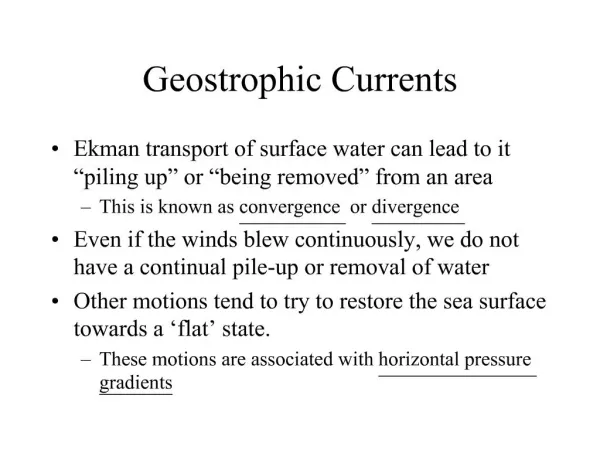
Geostrophic Currents
Geostrophic Currents. Lecture 12. OEAS-604. November 2, 2011. Outline: In-class Exercise Review of Baroclinic and Barotropic P.G.s Review of Geostrophic Balance Calculating Geostrophic Velocities Homework #3. η = 0.01 m. z = 0. σ t = 26. σ t = 26.5. σ t = 27. σ t = 27.5.

Geostrophic Currents
E N D
Presentation Transcript
Geostrophic Currents Lecture 12 OEAS-604 November 2, 2011 • Outline: • In-class Exercise • Review of Baroclinic and Barotropic P.G.s • Review of Geostrophic Balance • Calculating Geostrophic Velocities • Homework #3
η = 0.01 m z = 0 σt = 26 σt = 26.5 σt = 27 σt = 27.5 z = 1000m y-direction (+ into page) x-direction 10 km
Barotropic P.G. Baroclinic P.G. η = 0.01 m z = 0 σt = 26 σt = 26.5 σt = 27 σt = 27.5 z = 1000m y-direction (+ into page) x-direction 10 km
At surface, there is no baroclinic pressure gradient. So geostrophic velocity is simply: Flow is into the page (positive v) η = 0.01 m z = 0 σt = 26 σt = 26.5 σt = 27 σt = 27.5 z = 1000m y-direction (+ into page) x-direction 10 km
If there is no velocity at 1000m, this implies that the baroclinic and barotropic pressure gradients are equal. Baroclinic Velocity Barotropic Velocity Total Velocity 0 cm/s 10 cm/s 10 cm/s 0 cm/s -10 cm/s 10 cm/s Where positive v is into the page!
The Baroclinic Pressure Gradient can re-written in terms of the slope of the density interface using the reduced gravity. η ρ0 ζ ρ0+Δρ Using reduced gravity: Pressure Gradient can be represented as:
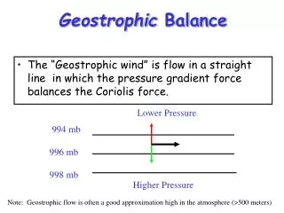
Geostrophic Balance: So, if we knew the pressure gradient exactly, it would be straight forward to calculate the velocity using the geostrophic balance. But, pressure gradient has both a baroclinic and barotropic component and so does the geostrophic velocity: Measuring changes in sea surface elevation can be very difficult.
Measuring density in the ocean is more straight forward. Taking vertical derivative of Geostrophic Balance gives: Thermal Wind Relationship In the absence of friction, vertical shear is the result of baroclinic pressure gradient. Integrate thermal wind relationship Geostrophic Balance: This is the contribution of the barotropic pressure gradient (uniform in z but hard to measure)
Geostrophic Balance: Because, we often don’t know the barotropic contribution to the pressure gradient, we assume that at some depth in the ocean, the flow goes to zero. This is called the depth of no motion. Oceanographers often assume that the depth of no motion occurs around a depth of 2000m.
Geostrophy and the Gulf Stream West East Useful rule of thumb: In northern hemisphere, warmer (less dense) water is to the right when looking down stream,
The Geostrophic Method for Calculating Currents has provided much of understanding of the currents in the interior of the Oceans, but this method must be applied with care: • Without accurate sea surface elevation, it only can provide “relative” currents and is subject to errors associated with the level of no motion. • Can’t be used in shallow water where there is no level of no motion and friction is important. • Provides only coarse resolution limited by CTD station spacing. • Does not apply where friction is important. • Breaks down near the equator where f~0. • May have errors due to non-steady processes such as internal waves, inertial oscillations, etc ….
Sea Surface Height Reflects Underlying Bathymetry Gravity vectors More Mass Less Mass Gravitational Vectors are shifted slightly by the uneven distribution of mass in the earth.
The Geoid is the an equipotential surface with respect to gravity, more or less corresponding to mean sea level. Local variations in gravity create minor hills and depressions (which range from -100 m to +60 m across the Earth) To plot geoid in Matlab type: load geoid; load coast figure; axesm robinson geoshow(geoid,geoidlegend,'DisplayType','texturemap') colorbar('horiz') geoshow(lat,long,'color','k') Gravitational acceleration is not constant everywhere on Earth!!
This is actually the sea surface height anomaly. So this is the deviation from the mean (which has large variations that reflect the underlying bathymetry).
Next Homework – Calculate the Geostrophic Velocity from the ARGO-CTD Data on the Class Website: ARGO_1.txt (38.081°N and -61.605°W) ARGO_2.txt (35.044°N and -61.107°W) Assume the depth of no motion is 1200 m. • Calculate the geostrophic velocity from the above data. • Be sure to specify what direction the current is flowing (N,S,E,W?). • What is the difference in sea surface between the two stations? Due one week from today: November 9, 2011