Download
1 / 35
440 likes | 947 Views
Currents without Friction Geostrophic, inertial and cyclostrophic balance. Pressure Gradient. ‘Friction’. Advection. Equations of motion - x-direction. Accn. Coriolis. When we examined the above equation, for the open ocean case,

E N D
Currents without FrictionGeostrophic, inertial and cyclostrophic balance
Pressure Gradient ‘Friction’ Advection Equations of motion - x-direction Accn Coriolis When we examined the above equation, for the open ocean case, we determined that from the order of magnitude of the terms, the two largest terms to be pressure gradient and Coriolis
Inertial Balance Frictionless equations Assume no pressure gradient i.e. Acceleration = Coriolis
Inertial Balance Inertial equations Re-arranging gives the Harmonic oscillator Solution
N t = 0 t = π /(2f) E t = 3π /( 2f ) t = π /f Inertial Motion Circular path due to centrifugal acceleration = U2 / r Rotation northern hemisphere - clockwise southern hemisphere – anti-clockwise
N E Inertial Period Inertial Period: Minimum at Poles; Maximum at equator = 24 h at latitude 30. Usually assumed to be the relaxation period
r y x Inertial Currents u u u u
Inertial Currents Inertial currents in the North Pacific in October 1987 (days 275–300) measured by a drifting buoy drogued at a depth of 15m. Positions were observed 10–12 times per day by the Argos system on NOAA polar-orbiting weather satellites and interpolated to positions every three hours. The largest currents were generated by a storm on day 277. Note these are not individual eddies. The entire surface is rotating. A drogue placed anywhere in the region would have the same circular motion. From van Meurs (1998).
Inertial Currents Example: A current meter array measured that currents in a region where the inertial period was 12 hours to be horizontally homogenous. At 12 noon the current was 0.1 ms-1 eastward. What is current speed and direction at 3pm, 6pm, 9pm and midnight. At what latitude were the currents measured ?
N t = 3 hrs E t = 6 hrs Inertial Currents t = 0, U = 0.1 t = 9 hrs
Cyclostrophic Balance Cyclostrophic Balance: Centrifugal force = Pressure gradient Examples: Water down plug hole Whirlpools tornadoes Rossby radius of deformation:
Geostrophic Equations • Assumptions • no acceleration, steady state, du / dt = dv / dt = dw / dt = 0 • w << u, v • The only external force is gravity • Friction negligible • Geostrophic Equations
B A Influence of pressure gradient In general, a slope in a water surface will generate a current down the slope:
B A Definition: Geopotential surface A geopotential surface is a horizontal surface i.e. gravity acts perpendicular to a geopotential surface Usually denoted by F F
geopotential surface isobars isopycnals increasing depth and density Barotropic circulation When isopycnals are parallel to isobars If F is parallel to isobars then there is no motion
Baroclinic circulation geopotential surface isobars isopycnals increasing depth and density When isopycnals intersect to isobars
Geopotential Distance geopotential surface isobars isopycnals increasing depth and density The change of geopotential is the potential energy/ unit mass gained by the parcel, or Definition: Geopotential distance – distance between two isobaric surfaces located at z1 and z2 Work required to raise a water parcel of mass M by a distance dz against gravity is Mgdz
Geostrophic Velocity F z Level of no motion isobar parallel to geopotential 1 2
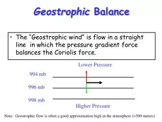
L H need to determine this pressure gradient Geostrophic Velocity
Sea SurfaceElevations At Kuroshio, the sea level difference is ~ 1 m in 100 km
Integrating But, Geopotential distance between z1 and z2 where pressures are p1 and p2 geopotential anomaly standard geopotential distance standard geopotential distance between z1 and z2 to calculate baroclinic pressure gradients We need to determine Units of geopotential distance: m2 / s2 or energy/unit mass
B A z1 z2 U1 P1 B1 A1 C1 z3 z4 U2 P2 B2 A2 C2
B A z1 z2 U1 P1 B1 A1 C1 z3 z4 U2 P2 B2 A2 C2
Station A: 41°55’N, 50°09’W m2/s2 Station B: 41°28’N, 50°09’W m2/s2 1000 m is the LNM; remember that 1 db = 104 Pa T S A B Depth (m) Depth (m) Depth (m)
0 26.56 26.88 200 27.19 26.90 = 27’ or 27 nautical miles apart 300 27.41 27.02 Vrel (m/s) 400 27.58 27.32 600 27.71 27.61 800 27.74 27.73 1000 27.78 27.77 A B Depth (m) Geopotential anomalies and relative velocities between A and B 27 n.m. x 1852 m/n.m. =50,000 m f = 9.7x10⁻⁵ s-1
Alongshore geopotential gradient Slope: 2.2 x 10⁻⁷
Geostrophic Method: Limitations • only the relative currents given (have to assume a level of no motion) • problems in shallower water • large spacing of stations (several 10’s of km) • cannot be used near the equator • acceleration and friction neglected
Example Two hydrographic stations, offshore Rottnest Island, obtained in mean water depths of 1000 m at a distance of 20 nautical miles apart in an east-west transect show that each water column consist of water of constant density. The western station has st=25.56 and the eastern st=26.62. What is the velocity between the two stations and its direction ? (assume that the ‘shorter’ water column is 1000m long).
Example B A 1000m Pressure at B: rgh = 1026.62 x 9.8 x 1000 Pressure at A: rgh = 1025.56 x 9.8 x h h = 1001.034 m pressure gradient = 1.034*1026.09*9.8/(20*1852) = 0.281 Velocity = 0.281/(1026.09*2*7.292*10-5*0.53) = 3.54 m/s
Cyclostrophic Balance We have considered 3 major forces: Pressure gradient Coriolis force Acceleration (centrifugal force) Geostrophic balance: Pressure gradient = Coriolis force Inertial Balance : Centrifugal force = Coriolis force Cyclostrophic Balance: Centrifugal force = Pressure gradient