Download
1 / 32
360 likes | 493 Views
Explore the simplification of basic equations for synoptic-scale motions through scale analysis. Learn about the significance of Rossby number, geostrophic balance, and vertical momentum equation in quasi-geostrophic motion.

E N D
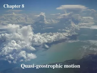
Chapter 8 Quasi-geostrophic motion
Scale analysis for synoptic-scale motions • Simplification of the basic equations can be obtained for synoptic scale motions. • Consider the Boussinesq system r is assumed to be constant in as much as it affects the fluid inertia and continuity. • Introduce nondimensional variables, ( ), and typical scales (in capitals) as follows: • (x, y) = L(x', y') z = Hz' t = (L/U)t' • (u,v) = U(u', v') w = Ww' p = Pp'; s = Ss '; and f = f0 f', • f0is a typical middle latitude value off.
The horizontal component of the momentum equation takes the nondimensional form where s'h denotes the operator (¶/¶x', ¶/¶y', 0) and Ro is the nondimensional parameter U/(f0L), the Rossby number. • Definition of scales => all (´)-quantities have magnitude ~ O(1). • Typical values of the scales for middle latitude synoptic systems are: L = l06 m, H = l04 m, U = 10 ms-1, P = 103 Pa (10 mb), s = gdT/T = 10*3/300 = 10 ms-2, r = 1 kg m-3 and f0 ~ 10-4 s. • Clearly, we can take P = ULf0. • Then, assuming that (WL/UH) ~ O(1), the key parameter is the Rossby number.
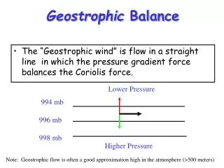
For synoptic scale motions at middle latitudes, Ro~ 0.l so that, to a first approximation, the D'u'h/Dt' can be neglected and the equation reduces to one of geostrophic balance. • In dimensional form it becomes We solve it by takingk^of both sides. This equation defines the geostrophic wind. Our scaling shows to be a good approximation to the total horizontal winduh.
As noted earlier, it is a diagnostic equation from which the wind can be inferred at a particular time when the pressure gradient is known. • In other words, the limit of as Ro 0 is degenerate in the sense that time derivatives drop out. • We cannot use the geostrophic equation to predict the evolution of the wind field. • If f is constant the geostrophic wind is horizontally nondivergent; i.e., sh× ug = 0 .
The difference between the horizontal wind and the geostrophic wind is called the ageostrophic wind: Now for Ro << 1, uh~ug while ua is of order Ro. A suitable scale for |ua| is URo. Because sh× ug = 0 , the continuity equation reduces to the nondimensional form (assuming that f is constant).
The second term of is important if a typical scale for w is U(H/L)Ro = 10-2 ms-1. the operator uh' × sh' in is much larger than ¶w'/¶z‘ . To a first approximation, advection by the vertical velocity can be neglected, both in the momentum and thermodynamic equations.
Two important results To a first approximation, advection by the vertical velocity can be neglected, both in the momentum and thermodynamic equations. Also the dominant contribution to uh' × sh'is u'g × sh' in quasi-geostrophic motion, advection is by the geostrophic wind.
Vertical momentum equation In nondimensional form, the vertical momentum equation is It is easy to check that SH/(ULf0) = 1 Ro(WH/UL) = Ro 2(H/L)2 = 10-6. Synoptic scale perturbations are in a very close state of hydrostatic balance.
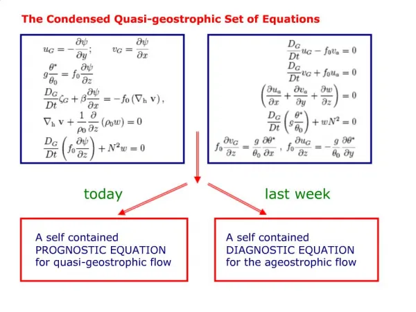
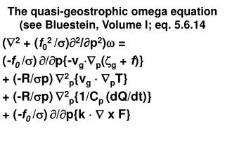
The governing equations for quasi-geostrophic motion in dimensional form an approximated form of the thermodynamic equation where at present f is assumed to be a constant.
A prediction equation for the flow at small Ro First derive the vorticity equation: Use: Taking k · ^ gives where zg = k ^ ug is the vertical component of relative vorticity computed using the geostrophic wind. If f is constant, .
Assume N2is constant of Take of Using
Assumes that f is a constant (then we can omit the single f in the middle bracket). • If the meridional displacement of air parcels is not too large, we can allow for meridional variations in f within the small Rossby number approximation - see exercise 8.1.
The quasi-geostrophic potential vorticity equation • Suppose that f = f0 + by, then where • This is an equation of fundamental importance in dynamical meteorology; it is the quasi-geostrophic potential vorticity equation • It states that the quasi-geostrophic potential vorticityq is conserved along geostrophically computedtrajectories. • It is the prognostic equation which enables us to calculate the time evolution of the geostrophic wind and pressure fields.
Solution procedure Write in the form
Suppose that we make an initial measurement of the pressure field p(x,y,z,0) at time t=0. • Calculate q(x,y,z,0) using • Calculated ug(x,y,z,0) using • Predict the distribution of q(x,y,z, Dt) using
Diagnose p(x,y,z,Dt) by solving the elliptic partial differential equation for p: • Diagnose ug(x,y,z,Dt) using • Repeat the process ...
Boundary conditions • In order to carry out the integrations, appropriate boundary conditions must be prescribed. • For example, for flow over level terrain, w = 0 at z = 0. Use and at z = 0
More on the approximated thermodynamic equation • When N is a constant, the nondimensional form of this equation is where and the Burger number the Rossby length • An important feature of quasi-geostrophic motion is the assumption that L ~ LR, or equivalently that B ~ 1.
When B ~ 1, The rate-of-change of buoyancy (and temperature) experienced by fluid parcels is associated with vertical motion in the presence of a stable stratification. • Since in quasi-geostrophic theory the total derivative D/Dt is approximated by ¶ /¶t+ug × s h , the rate-of-change of buoyancy is computed following the (horizontal) geostrophic velocity ug. • The vertical advection of buoyancy w¶ /¶zis negligible. • Thus quasi-geostrophic flows "see" only the stratification of the basic state characterized by N2 = (g/q)dq0/dz ---- this is independent of time; such flows cannot change the ‘effective static stability’ characterized locally by N2 + ¶s/¶z.
The quasi-geostrophic equation for a compressible atmosphere • The derivation of the potential vorticity equation for a compressible atmosphere is similar to that for a Boussinesq fluid. • The equation for the conservation of entropy, or equivalently, for potential temperature q, replaces the equation for the conservation of density: • Other changes are
The theory applies to small departures from an adiabatic atmosphere in whichq0(z) is approximately constant, equal toq*. For a deep atmospheric layer, the continuity equation must include the vertical density variation r0(z): The vorticity equation is The potential vorticity equation is
Quasi-geostrophic flow over a bell-shaped mountain • For steady flow (¶ /¶t º 0) the quasi-geostrophic potential vorticity equation takes the form ug× shq= 0. • Assume that f is a constant, • ug× shq= 0 is satisfied (e.g.) by solutions of the form q = f. • For these solutions, p satisfies or y is the geostrophic streamfunction (= p/rf). These solutions have zero perturbationpotential vorticity
Omit the zero subscript on f, and assume that N is a constant. Put Laplace’s equation Two particular solutions are: a uniform flow a source solution, strengthS at
Streamfunction equation is linear is a solution. In qg-flow because y= p/rf The vertical displacement of a fluid parcel, h is related to s by Since s is a constant on isentropic surfaces, the displacement of the isentropic surface from z = constant for the flow defined by y = -Uy - S/4pr is given (in dimensional form) by
The displacement of fluid parcels which, in the absence of motion would occupy the plane at z = 0 is hm = -S/(4pNR*2) R* = Nz*/f
is an isentropic surface of the quasi-geostrophic flow defined byy = -Uy - S/4pr. When S = 4pNR*2hmand z = f R*/N, y = -Uy - S/4pr represents the flow in the semi-infinite region z >= h of a uniform current U past the bell-shaped mountain with circular contours given by h(x,y). The mountain height is hmand its characteristic width is R*. In terms of hmetc., the displacement of an isentropic surface in this flow is
The vorticity changes in stratified quasi-geostrophic flow over an isolated mountain U A B O R* x
The streamline pattern in quasi-geostrophic stratified flow over an isolated mountain NH case The incident flow is distorted by the mountain anticyclone, but the perturbation velocity and pressure field decay away from the mountain (after R. B. Smith, 1979).
h2 - h1 -5 x 5 0 A B R* Height of the lowest isentrope above the topography in as a function of x. Unit scale equals the length of the four vertical lines in Fig. 8.1.
End of Chapter 8