Computers on Cruise Control
230 likes | 338 Views
This discussion explores the application of control theory in computer systems to optimize performance through adaptive systems. It covers the challenges of computer complexity, automation requirements, and fundamental control theory concepts such as feedback loops. The text provides insights on tuning systems to applications, monitoring performance metrics, adaptive management, and implementing feedback loops for desired outcomes. Examples and methods for creating difference equations to achieve performance goals are also discussed.

Computers on Cruise Control
E N D
Presentation Transcript
Computers on Cruise Control Creating Adaptive Systems with Control Theory Ricardo Portillo The University of Texas at El Paso raportil@miners.utep.edu
I’m going to talk about this The Ultimate Goal: Performance Performance Goals • Response Time; Throughput; Execution Time; CPU Utilization How do we increase performance? • Tune the application to the system • Tune the system to the application
Tuning the System to the Application • Determine the resource needs of the application • Determine what system parameters affect the application’s performance • Tune these parameters for optimal management of the application’s resources
The Problem: Computer Complexity • Computers and applications are growing larger • Systems are becoming more heterogeneous • Workload characteristics change rapidly
The Solution: Automation Requirements • Monitor if performance goals are being met • Adapt when performance changes • Guarantee that an adaptation will produce the desired effect at the right time
Analogous Scenario The cruise control in you car Requirements: • Monitordesired velocity is being met • Adapt accelerator when velocity changes • Guarantee that changes produce the desired velocity Cruise Control is implemented with Control Theory!
What is Control Theory? Control Theory is: • A branch of engineering and mathematics • Deals with systems that change over time Main Goal: Given a desired output from a system, manipulate system inputs to constantly achieve that output. Fundamental Concept: The Feedback Loop
The Feedback Loop • Desired/Measured Output: Performance Metrics • Control Input: Tuning Parameters • Disturbance Input: Workload Changes Disturbance Input Desired Output Measured Output Control Input Target System Controller
What’s Inside the Controller? • A difference equation describing the next output as a function of the current input and output: y(k+1) = a*y(k) +b*u(k) y(k+1) = Desired Performance y(k) = Current Performance u(k) = Parameter value to meet desired performance • Can be rewritten as: u(k) = [y(k+1) - a*y(k)] / b
Desired Output y(k+1) Controller u(k) = [y(k+1) - a*y(k)] / b Control Input u(k) Measured Output y(k) The Controller • Receive • Current performance y(k) • Desired performance y(k+1) • Produce • Required parameter value u(k)
Difference Equation Flexibility • Want to look more than one time step in the past? Use an ARX model: y(k+1) = a1y(k)+…+any(k-n+1)+b1u(k)+…+bmu(k-m+1) • Want more than one performance goal satisfied? Produce a separate equation for each performance goal: CPU(k+1) = a11CPU(k) + a12MEM(k)+b11u1(k)+b12u2(k) MEM(k+1) = a21CPU(k) + a22MEM(k)+b21u1(k)+b22u2(k)
Getting your Difference Equation • Determine your system scope • Choose your representative workload • Run your experiments: • Constantly change your parameters while workload is running • Keep track of the current parameter and performance values and of subsequent performance values • Perform a scatter plot analysis on your data to estimate the coefficients of your equation • Evaluate your equation and repeat if necessary
Server Example 1) Determine your system scope: - Performance Output = CPU Utilization (range 0-1) - Control Input = Number of Users (NU) (range 0-N) - CPU(k+1) = a*CPU(k) + b*NU(k) 2) Choose your representative workload: Some server benchmark (e.g. TPC-C) 3) Run experiments 1) Start up server benchmark 2) Record CPU(k) 3) Change NU(k) 4) Goto step 2 until benchmark ends
Experimental Results After least-squares regression analysis: CPU(k+1) = -0.087*CPU(k)+0.19*NU(k)
Server Feedback Loop Desired Output CPU(k+1) -> (e.g. CPU = 0.6) Control Input NU(k) Controller NU(k) = [0.6 + 0.087*CPU(k)] / 0.19 Server System Measured Output CPU(k)
Problem: Difference Equation may only work for the next timestep k+1 • Assume coefficients a = b = 1 => y(k+1) = y(k) + u(k) => u(k) = y(k+1) – y(k) • Assume at k = 1; y(k) = 1 and you want goal y(k+1) = 2 u(1)= 2 – 1 = 1 -> u(1)=1 will produce y(k+1)=2 ->Performance goal met at k=2 • What’s the value of y(k) at k=3? y(3) = y(2) + u(2) = 2 + 1 = 3 -> Goal not met at k=3! • As k grows ? y(k+1) = y(k) + 1 Performance metric will keep increasing until u(k) is remodified
Example that at least converges • Assume coefficients a = b = 0.5 =>y(k+1) = 0.5*y(k) + 0.5*u(k) => u(k) = [y(k+1) – 0.5*y(k)] / 0.5 • Assume k = 1; y(k) = 1 and you want goal y(k+1) = 2 u(1) = [2 – .5*1]/.5 = 3 -> u(1) = 3 will produce y(k+1) = 2 -> Performance goal met at k=2 • What’s the value of y(k) at k=3? y(3) = .5*y(2) + .5*u(2) = .5*2 + .5*3 = 2.5 Goal not met at k=3! • But… as k grows ? y(k+1) = {2.75, 2.87, 2.93, 2.96, 2.98,…} Performance metric converges to 3 if left unchecked • A system is stable if performance converges when control input changes • A system is accurate if it converges to the right performance value
Criteria for a Good Controller • Stability: Measured performance must converge to some value when control inputs are modified • Accuracy: Measured performance must converge to the performance goal when control inputs are modified • Short Settling: Measured performance must converge to the performance goal quickly when control inputs are modified
How can We Evaluate the Criteria? • Convert your difference equation into a non-recursive function by applying a Z-transform • Apply Control Theory theorems to your non-recursive function to assess: • If your equation always converges (Stability) • To what value will it converge (Accuracy) • How fast will it converge (Settling Time)
Advanced Control Theory • Gain Scheduling: Allows different controllers to be swapped at runtime. • Self-Tuning Regulators:Enables the creation of difference equations at runtime using recursive least-squares analysis. • Fuzzy Controllers: Applies heuristics written in symbolic logic when modifying control inputs. Used when system characterization is qualitative instead of quantitative.
Control Theory in Practice • Data Networks: Much work in data flow control for TCP protocols • Multimedia: Work on maintaining real-time performance constraints on data streams • Server and DB Software: Most popular application of CT recently. DB2 contains CT based performance tuning • Autonomic Computing Initiative: Applies holistic CT approach to large systems. Started in 2001 by IBM.
Future of CT in Computing • Apply CT not only for regulatory performance control but also to performance optimization (e.g. with Fuzzy controllers) • Automate the design of controllers (e.g. with Self-tuning regulators) • Incorporate artificial intelligence to create and manage adaptive systems at runtime (e.g. with agent based computing)
In Summary • Systems are becoming too complex to manage without automation • Control Theory provides a systematic method of integrating adaptation into a system • Control Theory is well established and easily maps to computing environments