Fuzzy Cruise Control
Fuzzy Cruise Control. Fuzzy Cruise Control. J. Yen and R. Langari, Fuzzy Logic: Intelligence, Control, and Information ( Prentice Hall, Upper Saddle River, New Jersey, 1999 ).

Fuzzy Cruise Control
E N D
Presentation Transcript
Fuzzy Cruise Control J. Yen and R. Langari, Fuzzy Logic: Intelligence, Control, and Information (Prentice Hall, Upper Saddle River, New Jersey, 1999). D. Simon, "Sum normal optimization of fuzzy membership functions," International Journal of Uncertainty, Fuzziness and Knowledge-Based Systems, Aug. 2002.
Fuzzy Cruise Control • = 12500 N • = 4 N / (m/s)2 • m = 1000 kg • fi = 1000 N (engine idle force,) • g = 9.81 m/s2
error = vref – v z=.2; w=1; t=0:.1:10; wd=w*sqrt(1-z*z); A=1; B=1; x=exp(-z*w*t).*(A*cos(wd*t)+B*sin(wd*t)); plot(t,x), hold on; plot(t, zeros(size(t)), 'r--')
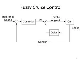
Fuzzy Cruise Control Error VehicleControl.m Change in Error Throttle Position Change
Default Membership Functions Error (meters/sec) PlotMem('DefaultMem.txt',2, [5 5], 1, 5)
Default Membership Functions Change in Error (meters/sec)
Default Membership Functions Throttle change (rad)
Input Membership Functions c = modal point, or “center” b– and b+ = half-widths 1 f(x) x b– c b+
j-th output membership function: j = modal point, or “center” j– and j+ = half-widths
Notation: fi1(x1) is membership of 1st input in i-th MF Similar for fk2(x2) Example: f11(x1) = 0 f21(x1) = 0.8 f31(x1) = 0.2 f41(x1) = 0 f51(x1) = 0 x1
If x1 is Ai and x2 is Bk, then y is Cj Firing level: So the fuzzy output when x1 fuzzy set i and x2 fuzzy set k is Point-wise sum of fuzzy outputs:
Centroid defuzzification with M rules: where j and Jj are the centroid and area of the j-th output fuzzy membership function
Substitute mj(y) from 4 pages earlier into the j equation on the previous page. Two pages of calculus and algebra later, Now use Theorem 4.1 in Jang to obtain the defuzzified output:
Fuzzy Cruise Control: VehicleControl.m 10 deg increase in road grade at t = 0
Fuzzy Controller Optimization • Gradient-based methods: Use the derivative of the tracking error with respect to the fuzzy MF parameters (Jang, Chapter 6) • “Home in” on a local optimum • Fast • Gradient-free methods (Jang, Chapter 7) • Genetic algorithms, etc. • Slow • No messy derivatives • “Global” optimization • General optimization (MF, number of rules, rule base, etc.)

