Download
1 / 31
320 likes | 398 Views
This tutorial delves into the intricacies of Z-transforms, their importance in digital regulation, and the relation between Laplace and Z-transforms. Topics covered include computation, stability analysis, precision, and discrete-time controller synthesis.

E N D
Theory of Z-transforms F. BOUVET 3rd POCPA Workshop, 21-23 May 2012, DESY
Answer to the following questions: What are Z-transforms ? Why are they so important ? How are they used for digital regulation ? Tutorial objective
Content Introduction Z-transforms Definition & properties Examples of Z-transforms Relation between Laplace and Z transforms Computation of the Z-transform of a signal from its Laplace transform Mapping from s-plane to z-plane Digitally controlled continuous-time systems Modelling of the plant to be controlled Open-loop and closed-loop transfer function Controller algorithm Analysis of closed-loop systems Stability of closed-loop systems and robustness Influence of the poles & zeros on the transient behavior Precision of closed-loop systems Discrete-time controller synthesis Emulation design Direct discrete-time design
x*(t) x(t) 1 t 0 Ts 2Ts 3Ts nTs Introduction • Reminder about Laplace transform: • Essential mathematical tool for continuous-time system & signal analysis ; stable or unstable • The Laplace transform X(s) of a continuous-time causal signal x(t) is given by • Case of discrete-time causal signals: • x(k)}, kℤ: Sequence of sampled values (= 0 k<0) • Ts: Sampling period (assumed constant) • : Dirac delta function • => The Laplace transform X*(s) of a discrete-time signal x*(t) is given by • (1) • Not a polynomial form…
Z-transform • Definition • With the change of variable in eq. (1), we derive the following expression • = definition of the Z-transform: • z ℂ for which X(z) converges • => Takes the form of a polynomial of the complex variable z • The Z-transform is the discrete-time counter-part of the Laplace transform • Essential tool for the analysis and design of discrete-time systems • Interpretation of the variable z-1 • From Laplace time-shift property, we know that is time advance by Ts second • Therefore corresponds to unit sample period delay
Z-transform • Properties of Z-transforms • - Linearity • - Shifting property • - Convolution • - Multiply by k property • - Final value
Z-transform 1 * k * * * * * 1 * * * * k * * * * * k * * * • Examples of Z-transforms • - Discrete impulse • - Discrete step • - Discrete ramp
Z-transform • Z-transform Table
Relation between Laplace and Z-transforms • X(s) X(z) ? • Case of signals having only simple poles • By sampling x(t), we obtain the following discrete sequence • From line 4 of the Z-transform table: • (2) • => A pole in X(s) yields a pole in X(z)
Relation between Laplace and Z-transforms • General case • (3) • Calculation of the residue at the pole of multiplicity m: • For a simple pole (m = 1): • An example of calculation will be given in the next chapter
Relation between Laplace and Z-transforms s z • Mapping from s-plane to z-plane • Since we can map the s-plane to the z-plane as below: • NB: 2 poles in the s-plane which imaginary part differ by map to the same pole in the z-plane • Bijective mapping between both planes =>
Relation between Laplace and Z-transforms s z • Mapping from s-plane to z-plane • Legend:
Digitally controlled continuous-time systems « Discretised » Plant Perturbations Ts Ts + DAC ADC _ Digital Controller Plant • Modelling of the plant to be controlled • Model of the DAC = Zero-order hold (ZOH) • Converts u(k) to u(t) by holding each sample value for one sample interval • The Laplace transform transfer function of the ZOH is • (4) • If H(s) has poles , then H(z) has poles . But the zeros are unrelated. NB: Delay introduced by the ZOH = Ts/2
Digitally controlled continuous-time systems • ways to calculate : • - Partial fraction decomposition + use z-transform table • - If has only simple poles, use Eq. (2): • - Use Eq. (3): • - Ask Matlab: Function ‘c2d’ • Syntax • sysd = c2d(sys,Ts) • Description • sysd = c2d(sys,Ts) discretizes the continuous-time LTI model sys using zero-order hold on the inputs and a sample time of Ts seconds.
Digitally controlled continuous-time systems • If • Open-loop transfer function: • Closed-loop transfer function: • Controller algorithm: • Transfer function of the digital controller • Hence • = Difference equation, where current output is dependent on current input and previous inputs and outputs
Digitally controlled continuous-time systems PWM signals Ts + PWM ADC _ Digital Controller Sampling Update of PWM signal duty cycle resulting from m(k) Output m(k) ADC + Computation time delay PWM clock Control delay = tc t kTs (k+1)Ts • Example: • Half bridge PWM converter • H(z) ? Controller output = modulation index (-1 < m < 1)
Digitally controlled continuous-time systems Ts Ts + ADC DAC _ + _ In this example and Modelling of the PWM converter The PWM can be modelled by a DAC with Using Eq. (3), with a double pole:
Analysis of closed-loop systems + _ Digital Controller « Discretised » Plant Unit Circle STABLE Poles of the closed-loop TF = Roots of the characteristic equation • Closed control loop performance criteria: • - Stability & robustness • - Static & dynamic behavior • The system behavior & stability is determined by the roots of the closed-loop TF • Stability of closed-loop systems • Mapping s-plane to z-plane • z-plane stable pole location Closed-loop transfer function:
Analysis of closed-loop systems 1/GM -1 w↗ ΦM • Robustness • Open-loop transfer function: • Phase margin ΦM : • Where is such that • Gain margin GM : • Where is such that • Typically: Matlab plots and margins Use functions ‘nyquist’ , ‘bode’ , ‘margin’
Analysis of closed-loop systems • Influence of the poles on the transient behavior • Will be illustrated with the step response analysis of a system CL(z) having only simple poles: • Step response @ sampling instants: • - Steady-state: • - Contribution of real poles : • Sum of • exponential terms • - Contribution of complex conjugate poles : • Oscillating • regime Dependent on pole locations => Damped oscillations => Undamped oscillations
Analysis of closed-loop systems Contribution of real poles Contribution of complex poles • Influence of the poles on the transient behavior • NB: Poles closer to origin Faster transient regime
Analysis of closed-loop systems s z • Particular case: 2nd order systems • A popular technique for controller design is pole placement. • A common strategy consists to derive the controller parameters from a pole placement such that the closed-loop behaves like a 2nd order system. • Continuous-time theory: • The design specifications imply • constrainsts on the cut-off frequency • and the damping ratio • Discrete closed-loops: • Pole mapping from s-plane to z-plane: Rise time (10% 90%): Peak overshoot: Settling time (to 1%): => condition for Ts
Analysis of closed-loop systems • Particular case: 2nd order systems • Influence of a zero • where z0 ℝ and • ( unitary static gain) • - Increasing overshoot when the zero is moving towards +1 Take care… • - The reference tracking performance can be improved by designing appropriate zeros in the closed-loop transfer function. Discrete step response
Analysis of closed-loop systems Perturbations Ts Ts + + DAC ADC + _ Digital Controller Plant • Precision of closed-loop systems • Same conclusions as for continuous-time closed-loops • - Precision versus the input • To achieve zero steady-state error, we require • at least 1 integrator (pole @ z =1) in the open-loop TF for a step input • at least 2 integrators in the open-loop TF for a ramp input • … • - Perturbation rejection • To reject disturbances of class N at least N+1 integrators in
Discrete-time controller synthesis Digital implemen-tation Controller discretization Continuous-time design Digital implemen-tation Plant discretization Controller design 2 main ways to synthesize discrete-time controllers: 1. Emulation design 2. Direct discrete-time design
Discrete-time controller synthesis • Emulation design • 1rst step: Continuous-time controller design. At this stage the sampling is ignored. But the control + ZOH delays should be taken into account ( preserve phase margin) • 2nd step: Discretization of the continuous-time controller (Followed by simulations to check Methods: performances) • - Approximate , i.e • - Pole-zero matching • 3rd step: Derivation of the controller algorithm (difference equation) • Approximation methods: • - Euler • - Tustin’s or bilinear approximation • Example: Discretization of a PI controller using Tustin’s approximation Matlab sysd = c2d(sys,Ts,’tustin’)
Discrete-time controller synthesis -1 1 -1 1 • Comparison between Euler and Tustin’s approx. • - Stability • - Mapping of the poles • Euler: => • Tustin: • => • To be compared to poles Euler Tustin Half- plane An unstable continuous-time system can be mapped to a stable discrete system Perfect correspondence
Discrete-time controller synthesis • Comparison between Euler and Tustin’s approx. • - Pole and zero locations not preserved Frequency response is changed • - Increasing the sampling frequency Smaller approximation errors • Example 1: Ts = 0.6 Ts = 0.06 => Better result with Tustin
Discrete-time controller synthesis is set so to obtain the same static gain • Comparison between Euler and Tustin’s approx. • Example 2: Ideal derivative • Other discretization method = Matched transform Euler:Filtering effect @ high frequencies Tustin: Magnitude ∞ when w /Ts Noise amplification @ high frequencies => Euler more appropriate for discretization of high-pass filters => Tustin more appropriate for discretization of low-pass filters Matlab sysd = c2d(sys,Ts,’matched’) No frequency distorsion => Well-adapted for the discretization of transfer functions including resonances (ex: notch filter, …)
Discrete-time controller synthesis • Direct discrete-time design • - A system controlled using an emulation controller always suffer the degradation of performance compared with its continuous-time counter-part • - To reduce the degree of degradation, very fast sampling can be needed, as • {ADC – Digital controller – DAC} should behave the same as the analogue controller (e.g. PID type) • Bad use of the potentialities of the digital controller • In this case, direct discrete-time design offers an alternative solution, since in this design the sampling is considered from the beginning of the design process • 1rst step: Discretization of the continuous-time plant (Cf. chapter 3) • 2nd step: Choice of controller type (PID, RST, …) and computation of the controller parameters using for example a pole placement method (Cf. chapter 4) • : Choice based on the bandwidth of the closed-loop system • 3rd step: Derivation of the controller algorithm (difference equation) • More in the next tutorials…
Questions • Thank you for your attention. • Questions ?