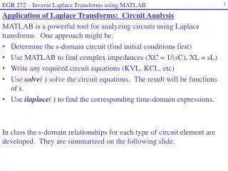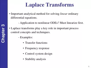
Laplace Transforms
Learn about Laplace transforms, a powerful tool for dynamics and control analysis. Convert mathematical operations, analyze block diagrams, and solve differential equations with ease using Laplace transforms. Explore examples and applications in process control and system stability.

Laplace Transforms
E N D
Presentation Transcript
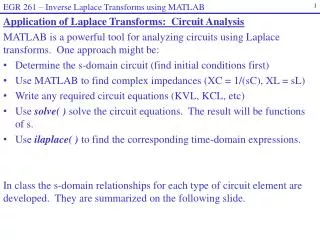
Laplace Transforms 1.Standard notation in dynamics and control (shorthand notation) 2. Converts mathematics to algebraic operations 3. Advantageous for block diagram analysis Chapter 3
Laplace Transform Example 1: Chapter 3 Usually define f(0) = 0 (e.g., the error)
Other Transforms etc. for Chapter 3 Note:
Table 3.1 Laplace Transforms for Various Time-Domain Functionsa f(t) F(s) Chapter 3
Table 3.1 Laplace Transforms for Various Time-Domain Functionsa f(t) F(s) Chapter 3
Table 3.1 Laplace Transforms for Various Time-Domain Functionsa (continued) f(t) F(s)
Example 3.1 Solve the ODE, First, take L of both sides of (3-26), Chapter 3 Rearrange, Take L-1, From Table 3.1 (line 11),
Example: system at rest (s.s.) Chapter 3 Step 1Take L.T. (note zero initial conditions)
Rearranging, Step 2a. Factor denominator of Y(s) Chapter 3 Step 2b. Use partial fraction decomposition Multiply by s, set s = 0
For a2, multiply by (s+1), set s=-1 (same procedure for a3, a4) Step 3.Take inverse of L.T. Chapter 3 (check original ODE) You can use this method on any order of ODE, limited only by factoring of denominator polynomial (characteristic equation) Must use modified procedure for repeated roots, imaginary roots
Laplace transforms can be used in process control for: 1. Solution of differential equations (linear) 2. Analysis of linear control systems (frequency response) 3. Prediction of transient response for different inputs Chapter 3
Factoring the denominator polynomial 1. Chapter 3 Transforms to e-t/3, e-t Real roots = no oscillation
2. Transforms to Complex roots = oscillation Chapter 3 From Table 3.1, line 17 and 18
Chapter 3 Let h→0, f(t) = δ(t) (Dirac delta) L(δ) = 1 Use L’Hopital’s theorem (h→0) If h = 1, rectangular pulse input
Difference of two step inputs S(t) – S(t-1) (S(t-1) is step starting at t = h = 1) By Laplace transform Chapter 3 Can be generalized to steps of different magnitudes (a1, a2).
One other useful feature of the Laplace transform is that one can analyze the denominator of the transform to determine its dynamic behavior. For example, if the denominator can be factored into (s+2)(s+1). Using the partial fraction technique Chapter 3 The step response of the process will have exponential terms e-2t and e-t, which indicates y(t) approaches zero. However, if We know that the system is unstable and has a transient response involving e2t and e-t. e2t is unbounded for large time. We shall use this concept later in the analysis of feedback system stability.
Other applications of L( ): A. Final value theorem “offset” Example 3: step response Chapter 3 offset (steady state error) is a. • Time-shift theorem • y(t)=0 t < θ
C. Initial value theorem Chapter 3 by initial value theorem by final value theorem
Chapter 3 Previous chapter Next chapter