Download
1 / 24
240 likes | 356 Views
Reconstruction of Heliospheric Magnetic Field Strength 1835-2014 180 Years of HMF B. Leif Svalgaard Stanford University AOGS ST04-06-A039 Sapporo, Aug. 1 st , 2014. Helsinki 1844-1912. Classic Method since 1846. Instruments ca. 1910. Weber. Gauss. 1830s. Modern Instrument.

E N D
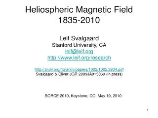
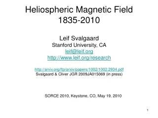
Reconstruction of Heliospheric Magnetic Field Strength 1835-2014 180 Years of HMF B Leif Svalgaard Stanford University AOGS ST04-06-A039 Sapporo, Aug. 1st, 2014
Helsinki 1844-1912 Classic Method since 1846 Instruments ca. 1910 Weber Gauss 1830s Modern Instrument Magnetic Recording over Time
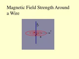
Typical Recording over 36 Hours 1 1 3 2 2 Three simultaneous features: 1: A Regular Daily Variation [it took 50 years to figure out the cause] 2: Shorter-term [~3 hour] fluctuations [‘substorms’ recognized in 1960s] 3: Large disturbances [‘geomagnetic storms’ explained in the 1960s] The complicated, simultaneous effects withstood understanding for a long time
Electric Current Systems in Geospace Different Current Systems Different Magnetic Effects BV Diurnal Var. BV2 FUV B nV2 Oppositely charged particles trapped in the Van Allen Belts drift in opposite directions giving rise to a net westward ‘Ring Current’. We can now invert the Solar Wind – Magnetosphere relationships…
‘Different Strokes for Different Folks’ • The key to using geomagnetism to say something about the sun is the realization that geomagnetic ‘indices’ can be constructed that respond differently to different solar and solar wind parameters, so can be used to disentangle the various causes and effects • In the last decade of research this insight (Svalgaard et al. 2003) has been put to extensive use and a consensus is emerging
24-hour running means of the Horizontal Component of the low- & mid-latitude geomagnetic field remove most of local time effects to show the Ring Current imprint: North H. Equator. South H. Latitude effect can be corrected for
Large HMF B results in large Kp B V n Kp
The IDV Geomagnetic Index • Since the daily variation is fairly regular from day to day we can eliminate it by considering the difference between consecutive days • Further suppression of the daily variation can be achieved by working only with the field during night hours or the average over a whole day • That led to the definition of the Interdiurnal Variability Index [IDV] as the unsigned difference between the geomagnetic field component on consecutive local nights • IDV is a Global index • IDV is a modern version of the u-measure
The u-measure Adolf Schmidt (1860-1944) Julius Bartels(1899-1964) N.A.F Moos (1859-1936) The u-measure was an index defined as the unsigned difference of the daily means of the horizontal component from one day to the next
IDV Derived from Many Stations (Observatories) Spread is due to different underground conductivity Early Version We normalize IDV by cos0.7(lat)
Relationship between HMF B and IDV Floor may a bit lower, like closer to 4.0 nT Also holds on timescales shorter than one year
Comparing the u-measure and IDV The IDV index and the u-measure track each other so well that either one can be used. We introduced the IDV based on only one hour per day because in the 19th century many stations did not observe at all hours throughout the day [not to speak about the night] so we wanted to see if only a few [as few as 1] hours worth of observations would be sufficient. As you can see, this hope seems fulfilled. The goal now is to extend the series to before 1872, potentially back to 1835 when Gauss and Co. initiated regular observations.
Other Ways to get the IDV Index Moos introduced the concept of ‘Summed Ranges’. Today we wouldn’t do it that way, but much of the early data and discussions center around concepts they used back then, so we go along. For each day, calculate the mean [of the data you have even if some hours are missing], the sum over all data points the absolute differences from that mean.
Lockwood et al. suggest to use the u-measure from HLS and ESK ?
Applying the methods described above we can reconstruct HMF B with Confidence: Lockwood et al. have conceded that their finding should be corrected and everybody now agree.
HMF B related to Sunspot Number The main sources of the equatorial components of the Sun’s large-scale magnetic field are large active regions. If these emerge at random longitudes, their net equatorial dipole moment will scale as the square root of their number. Thus their contribution to the average HMF strength will tend to increase as SSN1/2 (see: Wang and Sheeley [2003]; Wang et al. [2005]).
Schwadron et al. (2010) HMF B Model,with my set of parameters, including a ‘floor’ in B von Neumann: “with four parameters I can fit an elephant, and with five I can make him wiggle his trunk” This model has about eight parameters…
Combining Polar Faculae and Sunspot Areas can also give HMF B Andrés Muñoz-Jaramillo, 2012 MDI Counting Polar Faculae Threshold Filter
Conclusions • We can compute IDV, u back to 1835 • We can compute IDV, u from H and D • We can calibrate IDV in terms of HMF B measured by spacecraft since 1963 • We can thus estimate HMF B from IDV • We find that HMF B depends on the SSN½ • We can model HMF B from estimated polar faculae and the Schwadron Theory • All of these methods agree to ~10% • So we know HMF B for the past 180 years End
Abstract After C. F. Gauss and W. E. Weber's invention of the Magnetometer in 1833 systematic [e.g. hourly] measurements of the variation of the Earth's magnetic field were begun at several newly erected observatories around the World ["the Magnetic Crusade"]. These observations [greatly expanded] continue to this day. Magnetometers on the first spacecrafts to explore interplanetary space in 1962 showed that the, long hypothesized and then detected, solar wind carried a measurable magnetic field, which was soon identified as the main driver of disturbances of the magnetic fields observed at the Earth. Vigorous research during the last decade has shown that it is possible to 'invert' the causative effect of the magnetic field in near-Earth interplanetary space [the near-Earth Heliospheric Magnetic Field] and to infer with good accuracy the value of that field [and also of the solar wind speed and density] from the observed magnetic changes measured at the surface of the Earth. In this talk we describe the remarkable consensus reached by several researchers of the variation of the Heliospheric Magnetic Field (and thus of its source: the solar magnetic field) since the 1830s to today.