Variation Aware Gate Delay Models
This work presents a comprehensive approach to gate delay modeling, addressing the critical challenges of variability in integrated circuit (IC) design. Traditional modeling methods like TCAD and BSIM exhibit significant limitations in speed and scalability. Our finite point model leverages both accuracy and efficiency, enabling robust statistical timing analysis in modern nano-scale technologies. By incorporating process variations, our model facilitates faster simulations necessary for effective Monte Carlo analysis and enhances the reliability of IC designs. Future work aims to refine this method further and explore broader applications.

Variation Aware Gate Delay Models
E N D
Presentation Transcript
Variation Aware Gate Delay Models Dinesh Ganesan
Outline • Motivation • Background • Finite Point Model for gates • Results • Future work
Motivation Variability is an emerging design concern Design tools are just beginning to address variability and reliability concerns Right combination of better modeling and regular IC fabrics is the best way to resolve IC variability challenges
Background • Physical models • Based on physics of devices • Accurate • Very slow considering the number of transistors in today's design • Eg - TCAD • Empirical models • Device modeled with equations in various regions of operation. • Good accuracy • Slow for chip level simulations • Eg - BSIM3-the current industry standard, PSP, Gummel-Poon, Ebers Moll • Table model • Stored as lookup tables • Does not scale with change in circuit topology • Requires other models for characterization
BSIM • Given voltages at ports calculates the current/capacitance between the ports • Model them using equations with physical meaning • Parameter values obtained from the foundry/fab • Parameters grow exponentially in today's technology to address the emerging second order effects
Circuit Simulation • Circuit simulators like SPICE (Simulation Program with Integrated Circuit Emphasis) – a general purpose analog circuit simulator. • Solve nonlinear equations iteratively • Nodal analysis using Newton Raphson/Secant iteration for convergence • Use model file like BSIM for obtaining the voltage/current • Use of BSIM models for complete chip simulation takes months • Faster models of simulation required
130nm and above 90nm and below SSTA Variations • As transistor geometry decreases control of device parameters becomes difficult • Shift from Static timing analysis to Statistical timing analysis • Device model should be robust to process variations
Requirement • Fast simulation (including Monte Carlo) • Accurate • Model device • Robust to process variations
Current Source Model Model Gate Idc(Vi,Vo) – Current source Qx_y – Charge at x when y switches i – input o - output Idc – current captures static characteristics Q – charge – captures the dynamic characteristics
Idc(Vi,Vo) • Static I-V characteristics of a gate • Obtained using finite point model for pull-up (PUN) and pull down network (PDN) separately • Gate Idc(Vi,Vo) = PDN Idc(Vi,Vo) + PUN Idc(Vi,Vo)
Idc(Vi,Vo) – PUN/PDN Points required for the finite point model • Method similar to finite point model of transistor used, except that Id-Vi is nonlinear in this case • Two points for Id-Vo and five points for Id-Vi are sufficient to generate the complete IV • Points obtained by single DC simulation • Process variations – included in the IV • Continuous model in all regions required – continuous model for Idc-Vi Idc - Vo Idc - Vi
Idc(Vi,Vo) Simulation results for NAND2 Vin Vout
Q(Vi,Vo) • Calculate charge at input and output node based on switching at the nodes • Requires two transient simulations • Charge calculated by monitoring the current at the nodes during the simulation
PUN Vi Vo PDN Q(Vi,Vo) Calculation of Qo_i & Qi_i Transient simulation Idc model Vi Repeated for all values of Vi and Vo t1 t0
Q(Vi,Vo) Qo_i calculated from Idc model Qi_i Qo_i calculated from SPICE Idc
Q(Vi,Vo) Calculation of Qo_o & Qi_o PUN Transient simulation Idc model Vi Vo PDN Vo Repeated for all values of Vi and Vo t1 t0
Q(Vi,Vo) Qi_o Qo_o calculated from Idc model Qi_i Qo_i calculated from Idc model
Q(Vi,Vo) - approximation Qo_o -error Qo_o -approximated Qo_o -Actual Qo_i -approximated Qo_i -error Qo_i -Actual
Charge implementation in VerilogA Vin = V(tin,gr); Vout = V(tout,gr); Qi_i = f1(Vin,Vout); Qi_o = f2(Vin,Vout); Qo_i = f3(Vin,Vout); Qo_o = f4(Vin,Vout); I(tin,gr) <+ ddt(Qi_is); I(tout,gr) <+ ddt(Qo_os); I(tin,tout) <+ ddt(Qo_is); I(tout,tin) <+ ddt(Qi_os); tin tout Gate charge gr tin tout gr
Results Delay vs Input slew Output slew vs Input slew
Results Output voltage vs time Output current vs time
Advantages • Fast simulation • Accurate analysis • Process variations included with ease • Helps in fast Monte Carlo analysis