Download
1 / 26
260 likes | 411 Views
Parameterized Timing Analysis with General Delay Models and Arbitrary Variation Sources. Khaled R. Heloue and Farid N. Najm University of Toronto {khaled, najm}@eecg.utoronto.ca. Problem. Timing verification is a crucial step More pronounced in current technologies Types of variations

E N D
Parameterized Timing Analysis with General Delay Models and Arbitrary Variation Sources Khaled R. Heloue and Farid N. Najm University of Toronto {khaled, najm}@eecg.utoronto.ca
Problem • Timing verification is a crucial step • More pronounced in current technologies • Types of variations • Process variations are random statistical variations • Environmental variations are uncertain variations that are non-statistical • … cause circuit delay variations! • Parameterized Timing Analysis (PTA) • Delay is “parameterized” as a function of variations • Propagated in the timing graph to determine arrival times • Circuit delay becomes parameterized • Useful information: sensitivities, margins, distributions, yield
Previous Work • Statistical Static Timing Analysis (SSTA) • One type of PTA • Parameters are random variables withknown distributions • Gaussian?? • Different delay models • Linear, quadratic… • Different correlation models • Grid/Quad-tree, Principal Component Analysis (PCA) • Limitations: • Can not handle uncertain variables, i.e. nonstatistical variables • Some have difficulty in handling the Maxoperation efficiently • In nonlinear/non-Gaussian case
Previous Work • Multi-Corner Static Timing Analysis (MCSTA) • Is another type of PTA • Get a conservative bound on maximum(worst case) corner delay • Delay is parameterized using affine (linear) functions • Hyperplanes • Parameters can be random variables and/oruncertain variables • Limitations • Linear delay models • Does not follow well the spread of the circuit delay • Accuracy guaranteed only at the maximum corner delay • Sensitivities are not captured well
Our Approach • Propose a Parameterized Timing Analysis technique • Random parameters with arbitrary distributions • Uncertain non-statistical parameters • General class of delay models • Linear in circuit size (for linear and quadratic models) • Propose two methods to resolve the MAX operation • Using guaranteed upper/lower bounds • Using an approximation that minimizes the square of the error • Both methods preserve the nonlinearities of the delay model • Propose two applications: • MCSTA with linear/nonlinear models • SSTA with nonlinear models, random & uncertain variables
General Delay Models • To represent timing quantities, we will use a general class of delay models F • This class of nonlinear functions F has the following three properties: • F is closed under linear (and/or affine) operations • All functions in F are bounded • All functions in F can be maximized andminimized efficiently
General Delay Models – Cont’d • Property 1 • Property 2 • Property 3 • Guarantees overall efficiency of approach
Propagation • To propagate arrival times in the timing graph • SUM operation • MAX operation • SUM can be performed • By Property 1 of F • MAX is nonlinear • Bound the MAX using functions in F • Approximate the MAX using functions in F
MAX Operation • Let C = max(A,B) be the maximum of A and B and assume that A, B belong to F • C does not necessarily belong to F • We want to find
MAX Linear or Nonlinear?? • The nonlinearity of the MAX depends on the difference D, between A and B • Note that and that • MAX is linear when • Dmin ≥ 0 that is A dominates B C = A • Dmax ≤ 0 that is B dominates A C = B • MAX is nonlinear when Dmax ≥ 0 and Dmin ≤ 0
Bounding the MAX • C = B + max(D,0) and Dmax ≥ 0, Dmin ≤ 0 • Let Y = max(D,0) • Y does not belong to F since MAX is nonlinear
MAX Upper Bound • Yu is the best ceiling on Y and is exact at the extremes • Since Yu is a linear function of D, then
MAX Upper Bound – Cont’d • Since C = B + Y, then • Where
MAX Lower Bound – Cont’d • Lower bound on Y • Lower bound on C
MAX Approximation • Y = max(D,0) • Minimize:
MAX Approximation – Cont’d • Take the partial derivatives with respect to and • Set them to zero and solve for the variables • Simple expressions in Dmax and Dmin
Summary • Given a general class of nonlinear functions F with certain properties • If timing quantities • Then propagation (SUM & MAX) can be done while maintaining the same delay model • Bounds • LS Approximation • The MAX is “linearized” • Coefficients are simple functions of Dmin and Dmax • Independent of whether variables are random or uncertain • Distribution independent
Application 1 • Traditional STA • Need to check circuit timing at all process corners • Exponential number of runs • Multi-corner STA • Parameterize delay as a function of process/environmental parameters • Propagate once to get the maximum delay(also parameterized) • Determine the maximum/minimum cornerdelays efficiently • Apply our framework to MCSTA with linear/quadratic models
Linear/quadratic models • Timing quantities are expressed as follows: • Show that all properties hold • Linear/quadratic models survive linear(affine) operations • Bounded since -1 ≤ Xi ≤ 1 • Maximized efficiently (show in paper how this is done)
Results • 90nm library and following process parameters: • Vtn, Vtp, Ln, Lp • Characterized library to get delay sensitivities • Used ISCAS’85 circuits • Maximum delay at the maximum/minimum corners are computed using exhaustive STA • Maximum/minimum corner delays are determined using our approach (Bounds and LS-approximation) • Average errors:
Application 2 • SSTA with quadratic delay models • random parameters with arbitrary distributions (Gaussian, uniform, triangular, etc…) • uncertain non-random parameters varying inspecified ranges • Delay model:
The Three properties… • Surviving addition: • Bounded & can be maximized and minimized • The maximum and minimum of a quadratic function depends on whether the vertex is within the range or not (explained in the paper)
Results • In addition to Xr we use four global variables Xi • Truncated Gaussian, Uniform, and Triangular • 10%-20% deviation innominal delay • Compared our LS approach to Monte Carlo • Metrics: 95%-tile, 99%-tile, σ/μ • Avg error very small < 1%
Conclusion • Proposed the first Parameterized Timing Analysis technique • Random parameters with arbitrary distributions • Gaussian, uniform, triangular, etc… • Uncertain non-statistical parameters • Variables in ranges • General delay models (some restrictions) • Linear, quadratic, other… • Simple and accurate technique • Applied our framework to • Multi-corner STA with linear and quadratic models • Nonlinear (quadratic) SSTA with arbitrary distributions