Download
1 / 41
410 likes | 433 Views
Learn about the range, variance, standard deviation, coefficient of variation, interpretation of standard deviation, population and sample variance, approximation from grouped data, skewness, interquartile range and box plots, and the proportion of variability. Includes an example with height measurements of two teams.

E N D
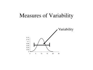
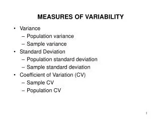
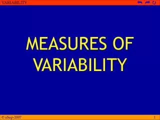
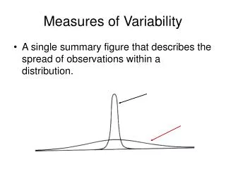
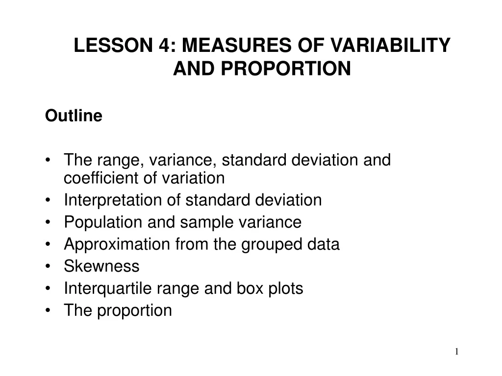
LESSON 4: MEASURES OF VARIABILITY AND PROPORTION Outline • The range, variance, standard deviation and coefficient of variation • Interpretation of standard deviation • Population and sample variance • Approximation from the grouped data • Skewness • Interquartile range and box plots • The proportion
MEASURES OF VARIABILITY: EXAMPLE • Heights of players of two teams in inches are as follows: Team I: 72,73,76,76,78, so mean=75, median=mode=76 Team II: 67,72,76,76,84, so mean=75, median=mode=76 • How about the variation?
MEASURES OF VARIABILITYRANGE • The first and simplest measure of variability is the range. • The range of a set of measurements is the numerical difference between the largest and smallest measurements. Range = Largest value - Smallest value
MEASURES OF VARIABILITYRANGE • Team I Range = 78-72 = inches • Team II Range = 84-67 = inches • So, Team I variation is a. less b. more
MEASURES OF VARIABILITYVARIANCE, STANDARD DEVIATION, CV • A major drawback of the range is that it uses only two extreme values, ignores all the intermediate values, and provides no information on the dispersion of the values between the smallest and largest observations. • On the other hand, variance / standard deviation / CV, uses all the values and provides information on the dispersion of the intermediate values • Computation of variance / standard deviation / CV requires computation of deviation from the mean
MEASURES OF VARIABILITYVARIANCE, STANDARD DEVIATION, CV • Team I deviations from the mean: (72-75)=-3, (73-75)=-2, (76-75)=1, ( - )= , ( - )=
MEASURES OF VARIABILITYVARIANCE, STANDARD DEVIATION, CV • Team I deviations from the mean: -3, -2, 1, , • From the property of mean (see Lesson 3, Slides 10-11), sum of deviations from the mean is zero. Check - 3 - 2 + 1 + + =
MEASURES OF VARIABILITYVARIANCE, STANDARD DEVIATION, CV • Sum of squared deviations from the mean is not necessarily 0 e.g., sum of squared deviations • Although sum of squared deviations increases if the dispersion increases, the sum depends on the number of measurements. So, mean squared deviations is a preferred measure of dispersion.
MEASURES OF VARIABILITYVARIANCE, STANDARD DEVIATION, CV • Variance is the mean squared deviation • For example, Team I variance
MEASURES OF VARIABILITYVARIANCE, STANDARD DEVIATION, CV • Standard deviation is the root mean squared deviation i.e., square root of variance. • So, Team I standard deviation
MEASURES OF VARIABILITYVARIANCE, STANDARD DEVIATION, CV • Coefficient of variation is the standard deviation divided by the mean. • So, Team I coefficient of variation
MEASURES OF VARIABILITYVARIANCE, STANDARD DEVIATION, CV • Why there are three similar terms? • In the above example, variance has unit inch2 • But, standard deviation has unit inch - the unit of the original data. So, standard deviation may sometimes be preferred over variance. • Coefficient of variation is dimension less. Hence, coefficient of variation is a useful quantity for comparing the variability in data sets having different standard deviations and different means.
MEASURES OF VARIABILITYVARIANCE, STANDARD DEVIATION, CV • Interpretation of standard deviation • It’s difficult to interpret • A higher standard deviation implies a greater variability • Standard deviation is widely used to approximate the proportion of measurements that fall into various intervals of values. This is specially true if the data has a bell-shaped distribution.
MEASURES OF VARIABILITYVARIANCE, STANDARD DEVIATION, CV • Interpretation of standard deviation • An empiricial rule states that if the data has a bell-shaped distribution, • approximately 68% measurements fall within one standard deviation of the mean i.e., between (mean-standard deviation) and (mean+standard deviation) • approximately 95% measurements fall within two standard deviations of the mean, and • virtually all the measurements fall within three standard deviations of the mean
Mean -3 -2 -1 +1 +2 +3 68.26% 95.44% 99.74% MEASURES OF VARIABILITYVARIANCE, STANDARD DEVIATION, CV
MEASURES OF VARIABILITYVARIANCE, STANDARD DEVIATION, CV • Interpretation of standard deviation • Example: suppose that the final marks has a bell-shaped distribution, with a mean of 75 and a standard deviation of 7. Then, • approximately 68% marks fall between (75-7)=68 and (75+7)=82. • approximately 95% marks fall between (75-27)=61 and (75+27)=89, and • virtually all the measurements fall between (75-37) =54 and (75+37)=96
POPULATION VARIANCE • The population variance is the mean squared deviation from the population mean: • Where 2stands for the population variance • is the population mean • N is the total number of values in the population • is the value of the i-th observation. • represents a summation
SAMPLE VARIANCE • The sample variance is defined as follows: • Where s2stands for the sample variance • is the sample mean • n is the total number of values in the sample • is the value of the i-th observation. • represents a summation
SAMPLE VARIANCE • Notice that the sample variance is defined as the sum of the squared deviations divided by n-1. • Sample variance is computed to estimate the population variance. • An unbiased estimate of the population variance may be obtained by defining the sample variance as the sum of the squared deviations divided by n-1 rather than by n. • Defining sample variance as the mean squared deviation from the sample mean tends to underestimate the population variance.
SAMPLE VARIANCE • A sample of monthly advertising expenses (in 000$) is taken. The data for five months are as follows: 2.5, 1.3, 1.4, 1.0 and 2.0. Compute the sample variance.
SAMPLE VARIANCE • An alternate formula for the sample variance: • Where s2stands for the sample variance • is the sample mean • n is the total number of values in the sample • is the value of the i-th observation. • represents a summation
SAMPLE VARIANCE • A sample of monthly sales expenses (in 000 units) is taken. The data for five months are as follows: 264, 116, 165, 101 and 209. Compute the sample variance using the alternate formula.
POPULATION/SAMPLE STANDARD DEVIATION • The standard deviation is the positive square root of the variance: Population standard deviation: Sample standard deviation:
POPULATION/SAMPLE STANDARD DEVIATION • Compute the sample standard deviation of advertising data: 2.5, 1.3, 1.4, 1.0 and 2.0 • Compute the sample standard deviation of sales data: 264, 116, 165, 101 and 209
POPULATION/SAMPLE CV • The coefficient of variation is the standard deviation divided by the means Population coefficient of variation: Sample coefficient of variation:
POPULATION/SAMPLE CV • Compute the sample coefficient of variation of advertising data: 2.5, 1.3, 1.4, 1.0 and 2.0 • Compute the sample coefficient of variation of sales data: 264, 116, 165, 101 and 209
SAMPLE VARIANCE APPROXIMATED FROM GROUPED DATA • Sample variance from grouped data: • Where s2stands for the sample variance • is the sample mean • n is the total number of observations • is the midpoint of the k-th class • is the frequency of the k-th class • represents a summation over all classes
SAMPLE VARIANCE APPROXIMATED FROM GROUPED DATA • Compute the sample variance of days to maturity of 40 investments from the following grouped data:
SAMPLE COEFFICIENT OF SKEWNESS • The sample coefficient of skewness: • Where SK stands for the coefficient of skewness • s is the sample standard deviation • is the sample mean • m is the sample median
SAMPLE COEFFICIENT OF SKEWNESS • Compute the sample coefficient of skewness of the advertising data: 2.5, 1.3, 1.4, 1.0 and 2.0 Mean, = 1.64 (see slide 20) Sample standard deviation, s = 0.6025 (see slides 20, 24) Median, m =
INTERQUARTILE RANGE AND BOX PLOTS • The interquartile range represents the range of the middle 50% observations and is the difference between the third quartile and the first. • The interquartile range • The range and interquartile range are combined in a box plot.
INTERQUARTILE RANGE AND BOX PLOTS • A box plot is used to graphically represent the data set. These plots involve five values: • the minimum value, S • the first quartile, • the second quartile or median, • the third quartile, • and the maximum value, L
INTERQUARTILE RANGE AND BOX PLOTS • Example: Construct a box plot with the following data which shows the assets of the 15 largest North American banks, rounded off to the nearest hundred million dollars: 111, 135, 217, 108, 51 , 98, 65, 85, 75, 75, 93, 64, 57, 56, 98
INTERQUARTILE RANGE AND BOX PLOTS • Sort the data in the ascending order (low to high): 51, 56, 57, 64, 65, 75, 75, 85, 93, 98, 98, 108, 111, 135, 217 • Find
INTERQUARTILE RANGE AND BOX PLOTS • If the median is near the center of the box, the distribution is approximately symmetric. • If the median falls to the left of the center of the box, the distribution is positively skewed. • If the median falls to the right of the center of the box, the distribution is negatively skewed. • If the lines are about the same length, the distribution is approximately symmetric. • If the line segment to the right of the box is larger than the one to the left, the distribution is positively skewed. • If the line segment to the left of the box is larger than the one to the right, the distribution is positively skewed.
THE PROPORTION • Population proportion is denoted by • The parameter is a number between 0 and 1 • Sample proportion is denoted by P • P serves as an estimator of and calculated as follows:
READING AND EXERCISES Lesson 4 Reading: Section 2-3, pp. 50-61 Exercises: 2-30, 2-37, 2-41