Download
1 / 36
360 likes | 395 Views
Learn about the four levels of measurement - nominal, ordinal, interval, and ratio - to understand how numbers represent data differently. Explore how each level allows for specific mathematical operations and analysis methods in research and statistics.

E N D
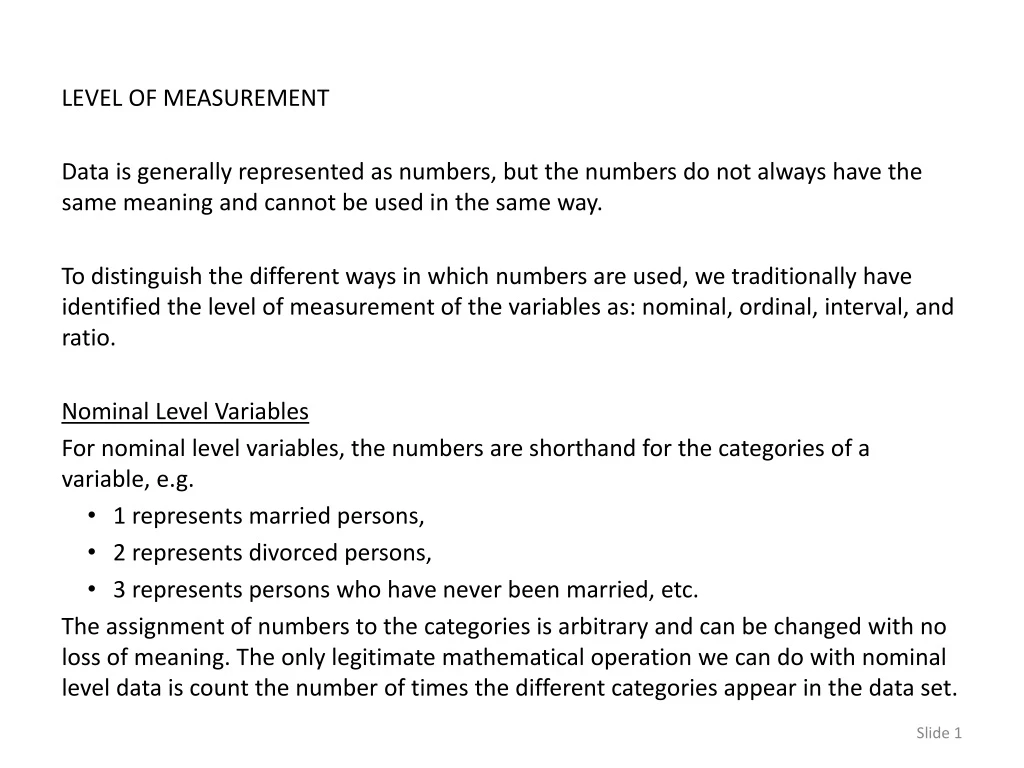
LEVEL OF MEASUREMENT Data is generally represented as numbers, but the numbers do not always have the same meaning and cannot be used in the same way. To distinguish the different ways in which numbers are used, we traditionally have identified the level of measurement of the variables as: nominal, ordinal, interval, and ratio. Nominal Level Variables For nominal level variables, the numbers are shorthand for the categories of a variable, e.g. • 1 represents married persons, • 2 represents divorced persons, • 3 represents persons who have never been married, etc. The assignment of numbers to the categories is arbitrary and can be changed with no loss of meaning. The only legitimate mathematical operation we can do with nominal level data is count the number of times the different categories appear in the data set.
Ordinal Level Variables Ordinal level variables are usually associated with labels as well, but the assignment of numbers to the categories is ordered, from low to high, e.g. • 1 is assigned to high school graduates, • 2 is assigned to junior college graduates, • 3 is assigned to college graduates, • 4 is assigned to graduates with a masters degree, etc. or from high to low: • 1 is assigned to graduates with a masters degree, • 2 is assigned to college graduates, • 3 is assigned to junior college graduates, • 4 is assigned to high school graduates , etc. The ordering of the numbers tracks the hierarchy of the labels. Though we can change the actual numbers used, the number assigned each higher level degree must consistently be a bigger number than what was used to represent lower ranked degrees (or a smaller number if ordered from high to low)
The legitimate mathematical operations we can perform on ordinal data is sorting or ranking, as well as counting. Interval Level Variables Interval level variables have the additional characteristic that the difference between numbers is the same for all possible combinations, e.g.: • the difference between 1 and 2 years of age is the same amount as the difference between 21 and 22 years of age, or 50 and 51, or 65 and 66. • the difference between a height of 60 inches and a height of 55 inches is the same amount of difference as a height of 72 inches and a height of 67 inches. For interval level variables, it is mathematically legitimate to do arithmetic (add, subtract, multiple, and divide) as well as count the values, and sort or rank the values. Ratio Level Variables Ratio level variables have the additional property of having a true zero value so that ratios between values are meaningful, but practically speaking, ratio level data is treated the same as interval level. The commonly cited example is temperature.
Quantitative and Categorical Variables The distinction between nominal and interval levels of variables is substantial. Computing an average marital status (treating a nominal level variable as interval) does not produce a meaningful result, and can be downright embarrassing. Presenting a count of all of the possible ages of the subjects in a data set (using only the nominal level property of an interval variable) does not communicate as much information as saying the average age was 27.5, with a range from 21 to 57. The differences in the use of data at these levels has led many authors to collapse the number of levels of measurement to two, substituting terms like: • quantitative or metric level instead of interval • categorical, qualitative, or non-metric instead of nominal In practice, ordinal level variable are sometimes treated as quantitative and at other times as categorical. The numeric codes for scale variables (1=disagree, 2=neutral, 3=agree) are generally treated as quantitative data and averaged. The numeric codes for year in school (1=freshman, 2=sophomore, 3=junior, 4=senior) are often not used, and comparisons are made using the categorical labels, e.g. the number (count) of seniors with some characteristic versus the number of juniors with the same characteristic.
When ordinal level variables are used as quantitative variables, we are emphasizing the rank order of the categories, e.g. 3 ranks higher than 2 or 1, and 2 ranks higher than 1. Since the ranks themselves are interval level data, it is argued that arithmetic on the ordinal values is acceptable. Multiple Variables Measuring the Same Construct The same construct can be represented by variables at different levels of measurement. Education can be represented as • years of school (quantitative), • diploma such as high school, college, or post-graduate (categorical, though we could come up with a numbering scheme that made it quantitative) The implication of these different representations is that we cannot base a correct conclusion on the name of the variable or the construct it represents. A correct understanding of a variable’s level of measurement requires that we look at the numbers in the data set and the coding scheme (numeric codes and labels) applied to the variable. The authors of the text for this course use the labels: quantitative and categorical. We will use their terminology in the first set of homework problems.
The introductory statement in the question indicates: • The data set to use (GSS2000R) • The task to accomplish (determining how the variable can be used) • The variable to use in the analysis: employment status [wrkstat] We will answer the question based on the way the data is presented in the SPSS data set. We will not consider changing the coding of the variable.
There are two statements for each problem. One or both might be correct.
In the Data View of the data editor, we see that wrkstatcontains numbers, but we cannot tell whether they are measures or codes.
Second, we look to see what numeric codes are used for missing data for the wrkstat row, in the Missing column. These are values that will not be used in the analysis and labels that we ignore in determining the level of measurement. First, to see what labels have been assigned to the variable, we click on the Variable View tab.
To see the values have been assigned labels, we look in the Variable View tab, and click in the right side of the cell on the row for wrkstat, in the column called Values.
When we clicked on the right end of the cell, the Value Labels dialog box opened. Ignoring the 0 and 9 which were coded as missing data, we see eight entries for work status.
To use the variable as quantitative, we examine the labels for order. I tried to think of them as describing the amount worked, but that clearly doesn’t work for retired, school, and keepinghouse. To close the dialog box, click on the OK button. Since I find no plausible order, the variable is categorical rather than quantitative.
The labels for this variable do not imply any order or rank. In fact the numeric codes could be reassigned to different categories with no loss of meaning. The statement that "Employment status can be used as a quantitative variable" is not correct and the check box is not marked. Since the variable has been assigned category labels in SPSS, the researchers who created the data set expected it to be used as a categorical variable. The statement that “Employment status can be used as a categorical variable" is correct and the check box is marked.
The second problem asks the same pair of questions about the variable number of hours worked in the past week [hrs1].
In the visible rows of the Data View, we see values that range from 38 to 60. Based on the variable label and the data values shown, my initial assessment is that this is a quantitative variable.
The variable hrs1 uses three numeric codes for missing data: -1, 98, and 99.
The only numbers assigned labels are the codes for missing data. There are no value labels for hrs1. Hrs1 is not a categorical variable.
Since the variable has not been assigned any category labels in SPSS, the researchers who created the data set expected it to be used as a quantitative variable. The statement that ""Number of hours worked in the past week" can be used as a quantitative variable" is correct and the check box is marked. Since the variable has not been assigned any category labels in SPSS, the researchers who created the data set expected it to be used as a quantitative variable. To use it as a categorical variable would require us to recode the variable into meaningful categories. The statement that ""Number of hours worked in the past week" can be used as a categorical variable" is not correct.
The third problem asks the same pair of questions about the self-employment [wrkslf].
In the Data View, we see very restricted options for values: 2 and 9.
The variable wrkslf uses three numeric codes for missing data: 0, 8, and 9.
If we eliminate the codes for missing data (0, 8, and 9), there are only two valid values (1 and 2). While labels have been assigned to the values for this variable which has only two categories, the variable can be considered ordered (and hence quantitative) if the categories are opposite, e.g. one category implies the possession of a characteristic that is different from the characteristic implied in the second category.
While labels have been assigned to the values for this variable which has only two categories, the variable can be considered ordered if the categories are opposite, e.g. one category implies the possession of a characteristic that is different from the characteristic implied in the second category. The statement that "Self-employment can be used as a quantitative variable" is correct and the check box is marked. Since the variable has been assigned category labels in SPSS, the researchers who created the data set expected it to be used as a categorical variable. The statement that ""Self-employment" can be used as a categorical variable" is correct and the check box is marked.
The fourteenth problem asks the same pair of questions about the how many in family earned money [earnrs].
In the first few rows of the Data View, we see that possible values for earnrs range from 0 through 3, and it is likely that there are higher values.
In the Variable View, we see that the variable earnrsuses only one numeric code for missing data: 9.
If we eliminate the code for missing data, there is only one value with a label, though we found other values for earnrs in the Data View. The labeling for this variable indicates that the highest code is used for 8 or more earners. This is done to eliminate higher number codes that have low frequencies. We can use earnrs as a categorical variable, but we would probably want to assign labels to the other values.
Assigning a label to a single value for a variable does not alter the order or rank of the other values of the variable. The variable can be treated as quantitative. The statement that ""How many in family earned money" can be used as a quantitative variable" is correct. Since the variable has been assigned category labels in SPSS, the researchers who created the data set expected it to be used as a categorical variable. The statement that ""How many in family earned money" can be used as a categorical variable" is correct.
The tenth problem asks the same pair of questions about the highest academic degree [degree].
The variable degree uses three numeric codes for missing data: 7, 8, and 9.
If we eliminate the codes for missing data (7, 8, and 9), there are five valid values. The are ordered by level of academic achievement and the number of years it takes to complete the degree. Graduate degrees take more years of school than bachelor degrees, which take more years of school than junior college degrees, etc.
While labels have been assigned to the values for this variable, the labels follow the order of the numeric codes. The order or rank to the response set supports the use of the variable as quantitative. The statement that "Highest academic degree can be used as a quantitative variable" is correct and the check box is marked. Since the variable has been assigned category labels in SPSS, the researchers who created the data set expected it to be used as a categorical variable. The statement that ""Highest academic degree" can be used as a categorical variable" is correct and the check box is marked.
When we have finished all of the questions, we click on the Submit at the bottom of the assignment.
BlackBoard asks us to verify that we wanted to submit the assignment. Click on the OK button.
Once the assignment is graded, we have the option to review the results. Click on the OK button.
Correct answers are marked with a green check. Incorrect answers are marked with a red X. Feedback is included to help you understand the reasons why the answers were correct or incorrect.