Download

1 / 55
550 likes | 784 Views
Lagrangian Descriptions of Turbulence. Greg Voth Wesleyan University, Middletown, CT, USA. Second Order Lagrangian Structure Function. A small Lagrangian inertial range may be visible. For R l of 815 the Eulerian structure functions would have well defined scaling ranges.

E N D
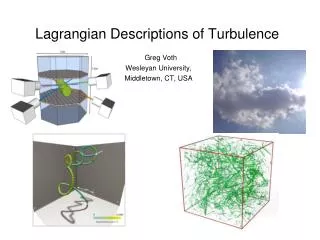
Lagrangian Descriptions of Turbulence Greg Voth Wesleyan University, Middletown, CT, USA
Second Order Lagrangian Structure Function • A small Lagrangian inertial range may be visible. • For Rl of 815 the Eulerian structure functions would have well defined scaling ranges. Biferale et al, Phys. Fluids 20:065103 (2008)
Second Order Lagrangian Structure Function • Lagrangian structure functions require larger Reynolds numbers to observe a scaling range if at all. • Despite the lack of clean scaling, the Lagrangian Kolmogorov constant C0~6 is very useful for stochastic modeling of turbulent mixing.
Higher Order Lagrangian Structure Functions K41 • Error bars are large for available data, but intermittency appears and deviations from K41 are larger than for the Eulerian velocity. They are even somewhat stronger than deviations for the passive scalar.
Acceleration Statistics with more recent data: intermittency corrections Rl0.13 Gulitski et al, JFM 2007
Lagrangian Tetrad Dynamics Xu et al, NJP 2008
Experimental Measurements of Particle Trajectories in Turbulence
Early Lagrangian Experiments • Richardson, 1922 • Balloons were released from Brighton England with labels asking a discoverer to return them with the landing location marked. • This data was used to justify Richardson’s law for two particle dispersion:
3D Particle Tracking Velocimetry • Developed by the Drakos group at ETH Zurich in the mid 1990s • Early implementations were limited to low Reynolds numbers (Rl~100) by available cameras (50 Hz frame rate). • Question: How many parameters are required to specify a camera’s viewpoint? Ott and Mann, JFM (2000)
Imaging requirements to resolve particle trajectories in intense turbulence • Spatial resolution: Number of pixels needed in one direction is So we would like 4000x4000 pixels • Temporal resolution: Frame period should be on the order of the Kolmogorov time so we would like frame rates in the kHz range. • Total Data Rate: 16 GB/sec
Silicon Strip Detectors for optical particle tracking Designed for charged particle detection at high energy physics collider experiments. 512 light sensitive strips with integrated amplifiers Reads out a 1D projection of the light intensity Up to 70,000 images per second
Silicon Vertex Detector during assembly of CLEO III at Cornell 447 silicon detectors arranged in 4 concentric cylinders Outer diameter: 30 cm Inner diameter: 8cm 43,000 channels ~100Hz event rate 4 MB/sec data rate from Silicon ~100 MB/sec from all detectors LHC produces ~1.8Gb/sec Richard Kass, Ohio State University
Strip Detectors for particle tracking in turbulence Tracer particles in the flow are optically imaged onto the detectors. Imaging volume is (2mm)3 512 channels 70kHz 35 MB/sec data rate per detector Two crossed imagers give resolution equal to 512x512 pixel imager: 5122*70kHz=18 Gb/sec
Trajectory measured with silicon strip detectors Tracer particles: 50 micron polystyrene spheres. 70,000 images per second on 4 strip detectors 30s event
Histogram of accelerations has higher probabilities of rare events than either the scalar gradient or the velocity gradients. Fit:
Acoustic Particle Tracking Mordant, Leveque and Pinton, PRL 2001, NJP 2004 2.5 MHz
3D PIV to obtain the velocity gradient tensor Zeff et al, Nature 2003
Probability Distribution of Energy Dissipation (strain rate squared)and Enstrophy (vorticity squared)
3D Particle Tracking Velocimetry Luthi et al, JFM 2005 Hoyer et al, Exp. In Fluids 2005 Mean eignevalues of the Cauchy Green Strain Tensor (Rl=50)
3D Particle Tracking Velocimetry with high speed cameras Ouellette et al, NJP 2005 Phantom v7 cameras 27 kHz at 256 x 256
Cameras that move with the mean velocity Ayyalasomayajula et al, PRL 2006
Experimental Problems • 3D particle tracking is always starved for light: • Illumination beam must be expanded to cover the detection volume. • Volume imaging requires small apertures. • Particles should be small enough to passively follow the flow. • High speed imaging means very little time to collect photons. • Images are never nice clean gaussian spots on a dark background • Stray reflections • Multiple reflections from tracer particles • Sometimes exactly focused particles only illuminate one pixel which greatly degrades position accuracy • At high seeding densities, images of particles overlap.
Recent Developments • Instrumented Particles • Particles with sensors for acceleration, pressure, etc. and radios to transmit data out of the flow. • Marked Particles • Particles with patterns created on their surface can be imaged to extract orientation in addition to position. • Index matched particles with tracers embedded allow standard 3DPTV to extract particle orientation.
Commercial Systems • TSI V3V • La Vision FlowMasterTomoPIV
Recent Developments • Instrumented Particles • Particle positions are found to a few microns from distances of 50 cm. • Calibrations drift. • A useful solution developed independently by several groups is dynamic calibration: Once you have an initial calibration of the position and orientation of the cameras, use real data with nonlinear optimization to adjust the calibration parameters to minimize mismatch between the rays from different cameras. • There is a reason plumbers are paid well…
Real-time Image Compression • Intermediate hardware between camera and computer • Input pixel brightness array, output a “vector” of (brightness, x, y) • Compression factors above 100 are routinely achieved. Compression Circuit Pixels Brightness & location Before, video ram limited data collection time to ~7 seconds=4Gb. Now with direct hard drive recording of compressed video, we can acquire data for ~7 days. Other compression schemes are possible, but the simple real-space basis seems to be nearly ideal for 3D particle tracking data.
Image Compression Circuit • 650 MB/sec data rate from the cameras • (Basler 1024X1280 pixels with 500 Hz frame rate). • Field Programmable IC: Altera® FPGA • Custom circuit board interfaces the FPGA with a camera • ~1 ½ year development and construction time by a master’s student • ~costs about $600
Summary of Experimental Particle Tracking Techniques • The wide range of scales in 3D turbulence precludes complete measurement of the flow, so one must choose either an Eulerian (fixed in space) or Lagrangian (particle tracking) measurements. • Rapid advances in imaging technology have led to rapid advances in capabilities of particle tracking systems.
Motion of Non-tracer particles in Turbulence Clouds are a major source of uncertainty in predictions of the rate of climate change expected. An unsolved problem is how water droplets in clouds rapidly grow from ~10 microns (where condensation becomes less important) to ~1mm (where they fall as rain). Droplet collisions are the growth mechanism and turbulence is believed to be an important ingredient.
Equation of motion for small particles at low particle Reynolds number For particles with a large density difference like water droplets in clouds, the external force (first term), fluid acceleration (second term) and Stokes drag (fourth term) dominate. In this case a single non-dimensional parameter defines the motion, the Stokes number:
If particles have size in the inertial range, then the acceleration variance should be only a function of particle diameter (d) and energy dissipation rate (e). The only combination of these with units of acceleration squared is e4/3d-2/3 What happens when the particles are large and neutrally buoyant? Particles larger than the Kolmogorov scale start to average over scales smaller than the particle diameter.
The Faxen model developed by Calzavarini et al (JFM 2009) predicts the particle acceleration is the average of the fluid acceleration over the particle size (for neutrally buoyant particles). Modeling particle size dependence: RNN and RLL are the transverse and longitudinal acceleration correlation functions. RNN and RLL are measured in Xu et al, PRL (2007).
Tracking Rods in 3D Turbulence • Shima Parsa, Wesleyan University • Nick Ouellette, Yale University Applications that require an understanding of rod dynamics include: • fibers for paper making • ice crystal dynamics in clouds • drag reduction
Sader 2008 Rod rotation rate is determined by the velocity gradients The rotation rate of an ellipsoid in Stokes flow was predicted by Jeffrey in 1922 =unit vector along the rod. =rod aspect ratio Tracking Rods allows a single particle measurement that contains information about the velocity gradient tensor!
At 3 Hz grid frequency Blum et al Physics of Fluids 2010 Flow between Two Oscillating Grids
Raw Data Rods are made of Nylon fibers d=300 μm (2h) L=1.5 mm (10h)a=5density=1.15 g/cm3 Rods are stained using fluorescent dye. Nd:YAG laser with 50 W average power is used for illumination.