Recall: Representation Changes:

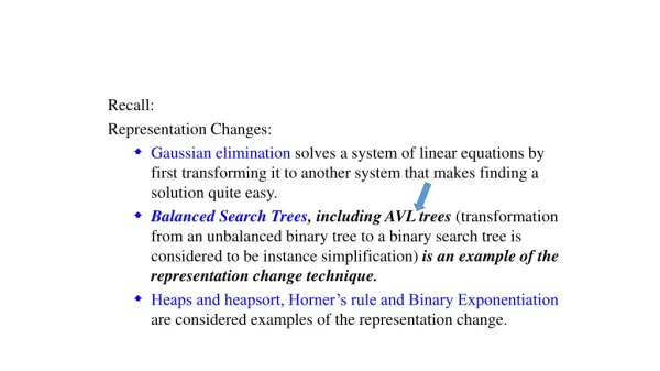
1. Recall: • Representation Changes: • Gaussian elimination solves a system of linear equations by first transforming it to another system that makes finding a solution quite easy. • Balanced Search Trees, including AVL trees (transformation from an unbalanced binary tree to a binary search tree is considered to be instance simplification) is an example of the representation change technique. • Heaps and heapsort, Horner’s rule and Binary Exponentiation are considered examples of the representation change.

2. AVL TreesThis data structure is named after two Russian scientists, G.M. Adelson-Velsky and E. M. Landis, who invented this data structure in 1962.Definition: An AVL tree is a binary search tree in which the balance factor of every node, which is defined as the difference between the heights of the node’s left and right subtrees, is either 0 or +1 or -1. (The height of the empty tree is defined as -1.)

3. Figure 6.2: The number beside each node indicates that node’s balance factor (= Height of left-subtree – Height of right-subtree for the node). 10 1 5 20 1 0 4 7 12 -1 0 1 2 8 0 0 (a) AVL tree.

4. Figure 6.2: The number beside each node indicates that node’s balance factor. factor = Lheight - Rheight 10 2 Right link Left link 5 20 0 0 4 7 factor Key’s value -1 1 Node’s size: 4 x ? bytes 2 (b) Binary search tree that is not an AVL tree. 8 0 0

5. If an insertion of a new node makes an AVL tree unbalanced, we transform the tree by a rotation. • Calculation of the different height between left and right subtrees at their parent node v: dheight(v) = ? • A rotation in an AVL tree is a local transformation of its subtree rooted at a node whose balance has become either +2 or -2; • if there are several sub nodes, we rotate the tree rooted at the unbalanced node that is the closest to the newly inserted leaf. • There are only four types of rotations: two of them are mirror images of the other two.

6. Figure 6.3 Four rotation types for AVL trees with three nodes. • Single R-rotation (on input 3, 2, 1) rightc c r 3 2 2 0 c r 2 g 1 3 R 1 0 0 g 1 0 Pattern: Factors are 2, 1. This needs single R-rotation at the node with factor 2.

7. Figure 6.3 Four rotation types for AVL trees with three nodes. • (b) Single L-rotation (on, input 1, 2, 3) left c 1 2 r -2 0 r c 2 g 1 3 -1 L 0 0 3 0 g Pattern: Factors are -2, -1. This needs single L-rotation at the node with factor -2.

8. Figure 6.3 Four rotation types for AVL trees with three nodes. • (c) Double LR-rotation (on input 3, 1, 2) g r 2 3 2 0 left r c c 3 1 1 LR 0 -1 0 right 2 r g 3 0 2 2 g 1 Pattern: Factors are 2, -1. This needs single L-rotation at the node with factor -1, and then R-rotation at the node with factor 2. c 1 0 0

9. Figure 6.3 Four rotation types for AVL trees with three nodes. • (d) Double RL-rotation (on input (1, 3, 2) r g 1 2 -2 0 right r c c 3 1 3 RL 0 1 0 r 2 g 1 0 -2 left g 2 -1 Pattern: Factors are -2, 1. This needs single R-rotation at the node with factor 1, and then L-rotation at the node with factor -2. c 3 0 0

10. Four Rotation Types: Pattern: Two adjacent nodes with factors are 2, 1. This needs single R-rotation at the node with factor 2. Pattern: Two adjacent nodes with factors are -2, -1. This needs single L-rotation at the node with factor -2. Pattern: Two adjacent nodes with factors are 2, -1. This needs single L-rotation at the node with factor -1, and then R-rotation at the node with factor 2. Pattern: Two adjacent nodes with factors are -2, 1. This needs single R-rotation at the node with factor 1, and then L-rotation at the node with factor -2.

11. Pattern: Two adjacent nodes with factors are 2, 1. • First rotation type: • Single right rotation (or R-rotation) • this rotation is performed after a new key is inserted into the left subtree of the left child of a tree whose root had the balance of +1 before the insertion.

12. Single R-rotation c r 2 r g c 1 g 1,-1 0 T3 T1 T2 T2 T3 T1 Figure 6.4 General form of the R-rotation in the AVL tree. A shaded node is the last one inserted. Pattern: Two adjacent nodes with factors are 2, 1. This needs single R-rotation at the node with factor 2

13. Pattern: Two adjacent nodes with factors are -2, -1. • 2. Single left rotation (or L-rotation) • This rotation is performed after a new key is inserted into the right subtree of the right child of a tree whose root had the balance of -1 before the insertion.

14. c r -2 c r g -1 g -1 0 T3 T1 T3 T2 T2 T1

15. Pattern: Two adjacent nodes with factors are 2, -1. • The second rotation type: • 3. Double left-right rotation (LR-rotation) • It is a combination of two rotations: • Perform the L-rotation of the left subtree of root r followed by the R-rotation of the new tree rooted at r. (see figure 6.5). • It is performed after a new key is inserted into the right subtree of the left child of a tree whose root has the balance of +1 before the insertion.

16. Pattern: Factors are 2, -1. This needs single L-rotation at the node with factor -1, and then R-rotation at the node with factor 2. • double LR-rotation g r 2 c r c -1 T4 T2 g 0 1, -1 T1 T3 T4 T2 T1 T3 or Figure 6.5 General form of the double LR-rotation in the AVL tree. A shaded node is the last one inserted. It can be either in the left subtree or in the right subtree or the root’s grandchild. or

17. Pattern: Two adjacent nodes with factors are -2, 1. • 4. The double right-left rotation (RL-rotation) • This is the mirror image of the double LR-rotation.

18. Pattern: Factors are -2, 1. This needs single R-rotation at the node with factor 1, and then L-rotation at the node with factor -2. • double RL-rotation g r -2 c r 0 c 1 T4 g 0 T1 T3 T2 1, -1 T1 T4 T2 T3 or • 4. The double right-left rotation (RL-rotation) • This is the mirror image of the double LR-rotation. or

19. Note that: The rotations are not trivial transformations. They can be done in constant time. They guarantee that a resulting tree is balanced They preserve the basic requirements of a binary search tree.

20. An example of constructing an AVL tree for a given list of numbers 5, 6, 8, 3, 2, 4, 7 by successive insertions is shown in following Figure 6.6. The parenthesized number of a rotation’s abbreviation indicates the root of the tree being reorganized.

21. Given list of numbers 5, 6, 8, 3, 2, 4, 7 by successive insertions in Figure 6.6, 5 5 0 5 -1 6 -2 0 L(at 5) -1 6 6 5 8 0 0 0 8 0 1 6 Pattern: Two adjacent nodes with factors are -2, -1. 1 5 8 0 3 0 5, 6, 8, 3, …

22. Given list of numbers 5, 6, 8, 3, 2, 4, 7 by successive insertions in Figure 6.6, 6 6 1 2 R(5) 5 3 8 8 0 2 0 0 2 3 5 1 0 0 2 0 5, 6, 8, 3, 2, … Pattern: Two adjacent nodes with factors are 2, 1.

23. Given list of numbers 5, 6, 8, 3, 2, 4, 7 by successive insertions in Figure 6.6, 6 0 5 2 L(3)R(6) 3 3 8 -1 6 0 -1 0 2 2 2 5 4 8 1 0 6 0 0 0 4 8 5 0 2 3 0 5, 6, 8, 3, 2, 4, … Pattern: Two adjacent nodes with factors are 2, -1. 2 4

24. Pattern: Two adjacent nodes with factors are -2, 1 and then -2, -1. Given list of numbers 5, 6, 8, 3, 2, 4, 7 by successive insertions in Figure 6.6, 5 0 5 -1 R(8)L(6) 0 3 3 7 6 0 0 -2 2 2 4 4 8 6 1 8 0 0 0 0 0 0 5 7 0 -2 6 5, 6, 8, 3, 2, 4, 7. 3 -1 7 2 4 8 Figure 6.6.

25. Single R-rotation c r 2 r g c 1 g 1,-1 0 T3 T1 T2 T2 T3 T1 Figure 6.4 General form of the R-rotation in the AVL tree. A shaded node is the last one inserted. Pattern: Two adjacent nodes with factors are 2, 1. This needs single R-rotation at the node with factor 2

26. Note that • In the initial tree in Figure 6.4, • all the keys of subtree T1 are smaller than its root c, • which is smaller than all the keys of subtree T2, • which are smaller than the root r, • which is smaller than all the keys of subtree T3. • And all the same relationships among the key values hold, as they must, for the balanced tree after the rotation. • In Figure 6.6, as you trace the algorithm operations, keep in mind that if there are several nodes with the ± 2 balance, the rotation is done for the tree rooted at the unbalanced node that is the closest to the newly inserted leaf.

27. How efficient are AVL trees? • As with any search tree, the critical characteristic is the tree’s height. • The tree’s height is bounded both above and below by logarithmic functions. • Specifically, the height h of any AVL tree with n nodes satisfies the inequalities • └ log2 n ┘ ≤ h < 1.4405 log2 (n + 2) – 1.3277. • These weird-looking constants are roundoffs of some irrational numbers related to Fibonacci numbers and the golden ratios. • The inequalities immediately imply that • the operations of search and insertion are Θ(log n) in the worse case. • Getting an exact formula for the average height of an AVL tree constructed for random lists of keys has prove to be difficult, but it is known [Knuth iii, p. 468].

28. Thus, searching in an AVL tree requires, on average, almost the same number of comparisons as searching in a sorted array by binary search. i.e., Θ(└ log2 n ┘ ) • The operation of key deletion in an AVL tree is • considerably more difficult than insertion, but fortunately • it turns out to be in the same efficiency class as insertion, i.e., logarithmic. (i.e., Θ(log n))

29. These impressive efficiency characteristics come at a price: • The drawbacks of AVL trees are • frequent rotations, the need to maintain balances for the tree’s nodes, and • overall complexity, especially of the deletion operation. • These drawbacks have prevented AVL trees from becoming the standard structure for implementing dictionaries. • At the same time, their underlying idea – that of rebalancing a binary search tree via rotations – has proved to be very fruitful and has led to discoveries of other interesting variations of the classical binary search tree.

30. Properties of AVL trees To implement an AVL tree, we maintain an extra field in each node: h[x] is the height of node x. As for any other binary search tree T, we assume that root[T] points to the root node. Prove that an AVL tree with n nodes has height O(log n). (Hint: Prove that in an AVL tree of height h, there are at least Fh nodes, where Fh is the hth Fibonacci number.)

31. Properties of AVL trees b. To insert into an AVL tree, a node is first placed in the appropriate place in binary search tree order. After this insertion, the tree may no longer be height balanced. Specifically, the heights of the left and right children of some node may differ by 2. Describe a procedure BALANCE(x), which takes a subtree rooted at x whose left and right children are height balanced and have heights that differ by at most 2, i.e., | h[right[x]] – h[left[x]] | ≤ 2, and alters the subtree rooted at x to be height balanced. (Hint: Use rotations.)

32. Properties of AVL trees c. Using part (b), describe a recursive procedure AVL-INSERT(x, z), which takes a node x within an AVL tree and a newly created node z (whose key has already been filled in), and adds z to the subtree rooted at x, maintaining the property that x is the root of an AVL tree. As in Tree-INSERT section, assume that key[z] has already been filled in and that left[z] = NIL and right[z] = NIL; also assume that h[z] = 0. Thus, to insert the node z into the AVL tree T, we call AVL-INSERT(root[T], z).

33. Properties of AVL trees d. Give an example of an n-node AVL tree in which an AVL-insert operation cause Ω(log n) rotations to be performed.

34. Balanced Search Trees - 2-3 Trees

35. 2-3 Trees • Another idea of balancing a search tree is to allow more than one key in the same node. • John Hopcroft (1970): a 2-3 tree implementation • Definition: • A 2-3 tree is a tree that can have nodes of two kinds: • 2-nodes and • 3-nodes.

36. 2-3 Trees • Definition: • A 2-3 tree is a tree that can have nodes of two kinds: • 2-nodes and • 3-nodes. • A 2-node contains a single key K and have two children: • the left child, which serves as the root of a subtree whose keys are less than K and • the right child, which serves as the root of a subtree whose keys are greater than k. (the classical binary search tree) • A 3-node contains two ordered keys K1 and K2 (k1 < K2) and has three children. • … 

37. 2-3 Trees • Definition: • A 2-3 tree is a tree that can have nodes of two kinds: • 2-nodes and • 3-nodes. • A 2-node contains a single key K and have two children: • … • A 3-node contains two ordered keys K1 and K2 (k1 < K2) and has three children. • The leftmost child, which serves as the root of a subtree with keys less than K1, • the middle child, which serves as the root of a subtree with keys between K1 and K2, and • the right most child, which serves as the root of a subtree with keys greater than K2.

38. Figure 6.7: Two kinds of nodes of a 2-3 tree. 2-node 3-node K K1 K2 <K1 (K1,K2) <K >K > K3

39. Definition: • The last requirement of the 2-3 tree is that • all its leaves must be on the same level. • That is, a 2-3 tree is always perfectly height-balanced: • the length of a path from the root of the tree to a leaf must be the same for every leaf. • It is this property that we allow more than one key in the same node of a search tree.

40. Searching for a given key K in a 2-3 tree is quite straightforward. • We start at the root. • If the root is a 2-node, we act as if it were a binary search tree: • we either stop if K is equal to the root’s key or • continue the search in the left or right subtree if K is, respectively, smaller or larger than the root’s key. • If the root is a 3-node, we know • after no more than two key comparisons whether the search can be stopped ( if K is equal to one of the root’s keys) or • in which of the root’s tree subtrees it needs to be continued.

41. Inserting a new key in a 2-3 tree is done as follows: • Insert a new key K in a leaf, except for the empty tree. • The appropriate leaf is found by performing a search for K. • If the leaf in question is a 2-node (i.e, it has only one key in the node), • we insert K there as either the first or the second key, depending on whether K is smaller or larger than the node’s old key. • If the leaf is a 3-node (i.e., insert K to form a 3-node),

42. Inserting a new key in a 2-3 tree is done as follows: • Insert a new key K in a leaf, except for the empty tree. • The appropriate leaf is found by performing a search for K. • If the leaf is a 3-node (i.e., insert K to form a 3-node), • we split the leaf in two: • the smallest of the three keys (two old ones and the new key) is put in the first leaf, • the largest key is put in the second leaf, • while the middle key is promoted to the older leaf’s parent. • (If the leaf happens to be the tree’s root, a new root is created for the middle key.) • Note that promotion of a middle key to its parent can cause the parent’s overflow (if it was a 3-node) and • hence can lead to sever node splits along the chain of the leaf’s ancestors.

43. An example of a 2-3 tree construction is given in Figure 6.8. Construction of a 2-3 tree for the list 9, 5, 8, 3, 2, 4, 7. 8 8 5 9 5 9 5 9 8 8 3 2 5 3 5 9 9

44. An example of a 2-3 tree construction is given in Figure 6.8. Construction of a 2-3 tree for the list 9, 5, 8, 3, 2, 4, 7. 8 2 8 3 2 4 5 3 9 2 5 9 9

45. An example of a 2-3 tree construction is given in Figure 6.8. Construction of a 2-3 tree for the list 9, 5, 8, 3, 2, 4, 7. 8 3 4 8 3 9 2 5 7 5 2 4 9 9

46. An example of a 2-3 tree construction is given in Figure 6.8. Construction of a 2-3 tree for the list 9, 5, 8, 3, 2, 4, 7. 8 3 7 8 3 9 2 5 4 7 5 2 4 9

47. An example of a 2-3 tree construction is given in Figure 6.8. Construction of a 2-3 tree for the list 9, 5, 8, 3, 2, 4, 7. 8 3 7 9 2 5 4 8 3 5 2 4 7 9

48. An example of a 2-3 tree construction is given in Figure 6.8. Construction of a 2-3 tree for the list 9, 5, 8, 3, 2, 4, 7. 8 3 5 7 2 4 9 5 5 8 3 2 4 7 9

49. For a 2-3 tree, we can implement each node having a 7 slots (i.e., a node consists of three keys and four pointer-addresses. However, the node has to split once it is full with three keys. Then the about implementation will be: for the list 9, 5, 8, 3, 2, 4, 7. 95, 9 5, 8, 9 8 8 8 5 9 3, 5 9 2,3,5 9 8 9 5 3 2

50. For a 2-3 tree, we can implement each node having a 7 slots (i.e., a node consists of three keys and four pointer-addresses. However, the node has to split once it is full with three keys. Then the about implementation will be: for the list 9, 5, 8, 3, 2, 4, 7. 8 3,8 3,8 2,3,5 9 2 5 9 2 4,5 9 4 7