Download

1 / 44
440 likes | 548 Views
This lecture covers essential methods for optimizing 3D mesh models, focusing on fairing (smoothing) and vertex relocation techniques to enhance visual appearance. Key approaches include centroid averaging for fairing and edge collapsing for 2D simplification, highlighting algorithms including minimizer computation, QEM updating, and the systematic reduction of vertex counts. It also addresses registration challenges in aligning models, including transformations using translation and rotation matrices, ensuring the structural integrity of the shape during modification processes.

E N D
CSE 554Lecture 5: Alignment Fall 2011
Review • Fairing (smoothing) • Relocating vertices to achieve a smoother appearance • Method: centroid averaging • Simplification • Reducing vertex count • Method: edge collapsing
Simplification (2D) • The algorithm • Step 1: For each edge, compute the best vertex location to replace that edge, and the QEM at that location. • Store that location (called minimizer) and its QEM with the edge.
Simplification (2D) • The algorithm • Step 1: For each edge, compute the best vertex location to replace that edge, and the QEM at that location. • Store that location (called minimizer) and its QEM with the edge. • Step 2: Pick the edge with the lowest QEM and collapse it to its minimizer. • Update the minimizers and QEMs of the re-connected edges.
Simplification (2D) • The algorithm • Step 1: For each edge, compute the best vertex location to replace that edge, and the QEM at that location. • Store that location (called minimizer) and its QEM with the edge. • Step 2: Pick the edge with the lowest QEM and collapse it to its minimizer. • Update the minimizers and QEMs of the re-connected edges.
Simplification (2D) • The algorithm • Step 1: For each edge, compute the best vertex location to replace that edge, and the QEM at that location. • Store that location (called minimizer) and its QEM with the edge. • Step 2: Pick the edge with the lowest QEM and collapse it to its minimizer. • Update the minimizers and QEMs of the re-connected edges. • Step 3: Repeat step 2, until a desired number of vertices is left.
Simplification (2D) • The algorithm • Step 1: For each edge, compute the best vertex location to replace that edge, and the QEM at that location. • Store that location (called minimizer) and its QEM with the edge. • Step 2: Pick the edge with the lowest QEM and collapse it to its minimizer. • Update the minimizers and QEMs of the re-connected edges. • Step 3: Repeat step 2, until a desired number of vertices is left.
Simplification (2D) • Step 1: Computing minimizer and QEM on an edge • Consider supporting lines of this edge and adjacent edges • Compute and store at the edge: • The minimizing location p • QEM of p • QEM coefficients (a, b, c) Stored at the edge:
Simplification (2D) • Step 2: Collapsing an edge • Remove the edge and its vertices • Re-connect two neighbor edges to the minimizer of the removed edge • For each re-connected edge: • Increment its coefficients by that of the removed edge • The coefficients are additive! • Re-compute its minimizer and QEM Collapse : new minimizer locations computed from the updated coefficients
Review • Fairing (smoothing) • Relocating vertices to achieve a smoother appearance • Method: centroid averaging • Simplification • Reducing vertex count • Method: edge collapsing
Registration • Fitting one model to match the shape of another • Automated annotation • Tracking and motion analysis • Shape and data comparison Courtesy: Sowell et al. Courtesy: Schneider and Eisert
Registration • Challenges: global and local shape differences • Imaging causes global shifts and tilts • Requires alignment • The shape of the organ or tissue differs in subjects and evolve over time • Requires deformation Brain outlines of two mice After alignment After deformation
Alignment • Registration by translation or rotation • The structure stays “rigid” under these two transformations • Also called isometric transformations (distance-preserving) • Accounts for shifts and tilts in imaging Before alignment After alignment
Transformation Math • Translation • Vector addition: • 2D: • 3D:
Transformation Math • Rotation • Matrix product: • 2D: • Rotate around the origin! • To rotate around another point q: y x
Transformation Math • Rotation • Matrix product: • 3D: z y Around X axis: x Around Y axis: Around Z axis:
Transformation Math • Properties of a rotational matrix • Orthonormal (orthogonal and normal): • Examples: • Easy to invert: • Any orthonormal matrix represents a rotation
Transformation Math • Properties of a rotational matrix • The rotation angle can be obtained from the trace of the matrix • Trace: sum of diagonal entries • 2D: • 3D: • αis the angle of rotation around the rotation axes • True for rotation around any axes (not just X,Y,Z) • The larger the trace, the smaller the rotation angle
Transformation Math • Eigenvectors and eigenvalues • Let M be a square matrix, v is an eigenvector and λ is an eigenvalue if: • Intuitively, if M represents a transformation, an eigenvector is invariant (up to scale) under the transformation. • There are at most m distinct eigenvalues for a m by m matrix • Any scalar multiples of an eigenvector is also an eigenvector (with the same eigenvalue).
Alignment • Input: two models represented as point sets • Source and target • Output: locations of the translated and rotated source points Source Target
Alignment • Method 1: Principal component analysis (PCA) • Aligning principal directions • Method 2: Singular value decomposition (SVD) • Optimal alignment given prior knowledge of correspondence • Method 3: Iterative closest point (ICP) • An iterative SVD algorithm that computes correspondences as it goes
Method 1: PCA • Compute a shape-aware coordinate system for each model • Origin: Centroid of all points • Axes: Directions in which the model varies most or least • Transform the source to align its origin/axes with the target
Method 1: PCA • Computing axes: Principal Component Analysis (PCA) • Consider a set of points p1,…,pn with centroid location c • Let P be a matrix whose i-th column is vector pi – c • 2D (2 by n): • 3D (3 by n): • Build the covariance matrix: • 2D: a 2 by 2 matrix • 3D: a 3 by 3 matrix
Method 1: PCA • Computing axes: Principal Component Analysis (PCA) • Eigenvectors of M represent principal directions of shape variation • The eigenvectors form orthogonal axes (2 vectors in 2D; 3 vectors in 3D) • Note they are “un-signed”: lacking an orientation. • Eigenvalues indicate amount of variation along each eigenvector • Eigenvector with largest (smallest) eigenvalue is the direction where the model shape varies the most (least) Eigenvector with the smallest eigenvalue Eigenvector with the largest eigenvalue
Method 1: PCA • PCA-based alignment • Let cS,cT be centroids of source and target. • First, translate source to align cS with cT: • Next, find rotation R that aligns two sets of PCA axes, and rotate source around cT: • Combined:
Method 1: PCA • Rotational alignment of two sets of oriented axes • Let A, B be two matrices whose columns are two sets of oriented axes • The axes are orthogonal and normalized • We wish to compute a rotation matrix R such that: • Notice that A and B are orthonormal, so we have:
Method 1: PCA • How to orient the PCA axes? • Observing the right-hand rule • There are 2 possible orientation assignments in 2D, and 4 in 3D 1st eigenvector 2nd eigenvector 3rd eigenvector
Method 1: PCA • Computing rotation R • Fix the orientation of the target axes. • For each orientation assignment of the source axes, compute R • Pick the R with smallest rotation angle (by checking the trace of R) Smaller rotation Larger rotation
Method 1: PCA • Limitations • Centroid and axes are affected by noise Noise Axes are affected PCA result
Method 1: PCA • Limitations • Axes can be unreliable for circular objects • Eigenvalues become similar, and eigenvectors become unstable PCA result Rotation by a small angle
Method 2: SVD • Optimal alignment between corresponding points • Assuming that for each source point, we know where the corresponding target point is
Method 2: SVD • Formulating the problem • Source points p1,…,pn with centroid location cS • Target points q1,…,qn with centroid location cT • qi is the corresponding point of pi • After centroid alignment and rotation by some R, a transformed source point is located at: • We wish to find the R that minimizes sum of pair-wise distances:
Method 2: SVD • An equivalent formulation • Let P be a matrix whose i-th column is vector pi – cS • Let Q be a matrix whose i-th column is vector qi – cT • Consider the cross-covariance matrix: • Find the orthonormal matrix R that maximizes the trace:
Method 2: SVD • Solving the minimization problem • Singular value decomposition (SVD) of an m by m matrix M: • U,V are m by m orthonormal matrices (i.e., rotations) • W is a diagonal m by m matrix with non-negative entries • The orthonormal matrix (rotation) is the R that maximizes the trace • SVD is available in Mathematica and many Java/C++ libraries
Method 2: SVD • SVD-based alignment: summary • Forming the cross-covariance matrix • Computing SVD • The rotation matrix is • Translate and rotate the source: Translate Rotate
Method 2: SVD • Advantage over PCA: more stable • As long as the correspondences are correct
Method 2: SVD • Advantage over PCA: more stable • As long as the correspondences are correct
Method 2: SVD • Limitation: requires accurate correspondences • Which are usually not available
Method 3: ICP • The idea • Use PCA alignment to obtain initial guess of correspondences • Iteratively improve the correspondences after repeated SVD • Iterative closest point (ICP) • 1. Transform the source by PCA-based alignment • 2. For each transformed source point, assign the closest target point as its corresponding point. Align source and target by SVD. • Not all target points need to be used • 3. Repeat step (2) until a termination criteria is met.
ICP Algorithm After PCA After 1 iter After 10 iter
ICP Algorithm After PCA After 1 iter After 10 iter
ICP Algorithm • Termination criteria • A user-given maximum iteration is reached • The improvement of fitting is small • Root Mean Squared Distance (RMSD): • Captures average deviation in all corresponding pairs • Stops the iteration if the difference in RMSD before and after each iteration falls beneath a user-given threshold
More Examples After PCA After ICP
More Examples After PCA After ICP