Download
1 / 42
440 likes | 577 Views
The following slides have been adapted from http://www.tm4.org/ to be presented at the Follow-up course on Microarray Data Analysis (Nov 20-24 2006, PICB Shanghai) by Peter Serocka. Analysis of Multiple Experiments TIGR Multiple Experiment Viewer (MeV). Exp 1. Exp 2. Exp 3. Exp 4. Exp 5.

E N D
The following slides have been adapted from http://www.tm4.org/ to be presented at the Follow-up course on Microarray Data Analysis (Nov 20-24 2006, PICB Shanghai) by Peter Serocka
Analysis of Multiple ExperimentsTIGR Multiple Experiment Viewer (MeV)
Exp 1 Exp 2 Exp 3 Exp 4 Exp 5 Exp 6 Gene 1 Gene 2 Gene 3 Gene 4 Gene 5 Gene 6 The Expression Matrix is a representation of data from multiple microarray experiments. Each element is a log ratio (usually log 2 (Cy5 / Cy3) ) Black indicates a log ratio of zero, i. e., Cy5 and Cy3 are very close in value Green indicates a negative log ratio , i.e., Cy5 < Cy3 Gray indicates missing data Red indicates a positive log ratio, i.e, Cy5 > Cy3
1.5 -0.8 1.8 0.5 -0.4 -1.3 1.5 0.8 Expression Vectors -Gene Expression Vectors encapsulate the expression of a gene over a set of experimental conditions or sample types. Log2(cy5/cy3)
Expression Vectors As Points in‘Expression Space’ Exp 1 Exp 2 Exp 3 G1 -0.8 -0.3 -0.7 G2 -0.7 -0.8 -0.4 G3 Similar Expression -0.4 -0.6 -0.8 G4 0.9 1.2 1.3 G5 1.3 0.9 -0.6 Experiment 3 Experiment 2 Experiment 1
Distance and Similarity -the ability to calculate a distance (or similarity, it’s inverse) between two expression vectors is fundamental to clustering algorithms -distance between vectors is the basis upon which decisions are made when grouping similar patterns of expression -selection of a distance metric defines the concept of distance
Exp 1 Exp 2 Exp 3 Exp 4 Exp 5 Exp 6 x1A x2A x3A x5A Gene A x4A x6A Gene B x1B x2B x3B x4B x5B x6B 6 6 • Manhattan: i = 1 |xiA – xiB| Distance: a measure of similarity between genes. p1 • Some distances: (MeV provides 11 metrics) • Euclidean: i = 1(xiA - xiB)2 p0 3. Pearson correlation
Distance Metric: EuclideanPearson(r*-1) D D Distance is Defined by a Metric 1.4 -0.90 4.2 -1.00
Hierarchical Clustering (HCL) HCL is an agglomerative clustering method which joins similar genes into groups. The iterative process continues with the joining of resulting groups based on their similarity until all groups are connected in a hierarchical tree. (HCL-1)
g1 g1 g1 g8 g2 g8 g3 g4 g2 g2 g3 g4 g5 g4 g3 g5 g6 g5 g7 g6 g6 g7 g8 g7 Hierarchical Clustering g1 is most like g8 g4 is most like {g1, g8} (HCL-2)
g1 g1 g1 g8 g8 g8 g4 g4 g4 g2 g5 g2 g3 g3 g7 g5 g2 g5 g6 g7 g3 g7 g6 g6 Hierarchical Clustering g5 is most like g7 {g5,g7} is most like {g1, g4, g8} (HCL-3)
g1 g8 g4 g5 g7 g2 g3 g6 Hierarchical Tree (HCL-4)
Hierarchical Clustering During construction of the hierarchy, decisions must be made to determine which clusters should be joined. The distance or similarity between clusters must be calculated. The rules that govern this calculation are linkage methods. (HCL-5)
Agglomerative Linkage Methods • Linkage methods are rules or metrics that return a value that can be used to determine which elements (clusters) should be linked. • Three linkage methods that are commonly used are: • Single Linkage • Average Linkage • Complete Linkage (HCL-6)
Single Linkage Cluster-to-cluster distance is defined as the minimum distance between members of one cluster and members of the another cluster. Single linkage tends to create ‘elongated’ clusters with individual genes chained onto clusters. DAB = min ( d(ui, vj) ) where u Î A and v Î B for all i = 1 to NA and j = 1 to NB DAB (HCL-7)
Average Linkage Cluster-to-cluster distance is defined as the average distance between all members of one cluster and all members of another cluster. Average linkage has a slight tendency to produce clusters of similar variance. DAB = 1/(NANB) S S ( d(ui, vj) ) where u Î A and v Î B for all i = 1 to NA and j = 1 to NB DAB (HCL-8)
Complete Linkage Cluster-to-cluster distance is defined as the maximum distance between members of one cluster and members of the another cluster. Complete linkage tends to create clusters of similar size and variability. DAB = max ( d(ui, vj) ) where u Î A and v Î B for all i = 1 to NA and j = 1 to NB DAB (HCL-9)
Single Ave. Complete Comparison of Linkage Methods (HCL-10)
K-Means / K-Medians Clustering (KMC)– 1 G1 G2 G3 G4 G5 G6 G7 G8 G9 G10 G11 G12 G13 1. Specify number of clusters, e.g., 5. 2. Randomly assign genes to clusters.
G3 G6 G1 G8 G4 G5 G2 G10 G9 G12 G13 G11 G7 K-Means Clustering – 2 3. Calculate mean / median expression profile of each cluster. 4. Shuffle genes among clusters such that each gene is now in the cluster whose mean / median expression profile (calculated in step 3) is the closest to that gene’s expression profile. 5. Repeat steps 3 and 4 until genes cannot be shuffled around any more, OR a user-specified number of iterations has been reached. K-Means / K-Medians is most useful when the user has an a-priori hypothesis about the number of clusters the genes should group into.
Cluster Affinity Search Technique (CAST) -uses an iterative approach to segregate elements with ‘high affinity’ into a cluster -the process iterates through two phases -addition of high affinity elements to the cluster being created -removal or clean-up of low affinity elements from the cluster being created
G3 G13 G8 Empty cluster C1 G2 G14 G4 G12 G1 G5 G15 G9 G6 G11 G7 G10 Unassigned genes Affinity = a measure of similarity between a gene, and all the genes in a cluster. Threshold affinity = user-specified criterion for retaining a gene in a cluster, defined as %age of maximum affinity at that point Clustering Affinity Search Technique (CAST)-1 1. Create a new empty cluster C1. 2. Set initial affinity of all genes to zero 3. Move the two most similar genes into the new cluster. 4. Update the affinities of all the genes (new affinity of a gene = its previous affinity + its similarity to the gene(s) newly added to the cluster C1) ADD GENES: 5. While there exists an unassigned gene whose affinity to the cluster C1 exceeds the user-specified threshold affinity, pick the unassigned gene whose affinity is the highest, and add it to cluster C1. Update the affinities of all the genes accordingly.
REMOVE GENES: CAST – 2 6. When there are no more unassigned high-affinity genes, check to see if cluster C1 contains any elements whose affinity is lower than the current threshold. If so, remove the lowest-affinity gene from C1. Update the affinities of all genes by subtracting from each gene’s affinity, its similarity to the removed gene. 7. Repeat step 6 while C1 contains a low-affinity gene. G3 G13 G8 Current cluster C1 G2 G4 G6 G14 G12 G5 G9 G11 G7 G1 G10 G15 Unassigned genes 8. Repeat steps 5-7 as long as changes occur to the cluster C1. 9. Form a new cluster with the genes that were not assigned to cluster C1, repeating steps 1-8. 10. Keep forming new clusters following steps 1-9, until all genes have been assigned to a cluster
G9 G6 G8 G11 G4 G10 G11 G1 G2 G5 G7 G3 “Seed” gene G12 Currently unassigned genes Current cluster QT-Clust (from Heyer et. al. 1999) (HJC) -1 • Compute a jackknifed distance between all pairs of genes • (Jackknifed distance: The data from one experiment are excluded from both genes, and the • distance is calculated. Each experiment is thus excluded in turn, and the maximum distance • between the two genes (over all exclusions) is the jackknifed distance. This is a conservative • estimate of distance that accounts for bias that might be introduced by single outlier experiments.) 2. Choose a gene as the seed for a new cluster. Add the gene which increases cluster diameter the least. Continue adding genes until additional genes will exceed the specified cluster diameter limit. 3. Repeat step 2 for every gene, so that each gene has the chance to be the seed of a new cluster. All clusters are provisional at this point.
G7 G11 G4 G11 G8 G1 G1 G10 G2 G8 “Seed” gene G9 “Seed” gene G3 G7 G12 G5 4. Choose the largest cluster obtained from steps 2 and 3. In case of a tie, pick one of the largest clusters at random. QT-Clust – 2 G4 G9 G3 “Seed” gene Pick this cluster 5. All genes that are not in the cluster selected above are treated as currently unassigned. Repeat steps 2-4 on these unassigned genes. 6. Stop when the last cluster thus formed has fewer genes than a user-specified number. All genes that are not in a cluster at this point are treated as unassigned.
SOTA - 1 Self Organizing Tree Algorithm • Dopazo, J. , J.M Carazo, Phylogenetic reconstruction using and unsupervised growing neural network that adopts the topology of a phylogenetic tree. J. Mol. Evol. 44:226-233, 1997. • Herrero, J., A. Valencia, and J. Dopazo. A hierarchical unsupervised growing neural network for clustering gene expression patterns. Bioinformatics, 17(2):126-136, 2001.
SOTA - 2 SOTA Characteristics • Divisive clustering, allowing high level hierarchical structure to be revealed without having to completely partition the data set down to single gene vectors • Data set is reduced to clusters arranged in a binary tree topology • The number of resulting clusters is not fixed before clustering • Neural network approach which has advantages similar to SOMs such as handling large data sets that have large amounts of ‘noise’
SOTA - 3 SOTA Topology Centroid Vector Parent Node ap Members as aw Winning Cell Sister Cell a* = migration factor (as < ap < aw)
SOTA - 4 Adaptation Overview -each gene vector associated with the parent is compared to the centroid vector of its offspring cells. -the most similar cell’s centroid and its neighboring cells are adapted using the appropriate migration weights.
SOTA - 5 -following the presentation of all genes to the system a measure of system diversity is used to determine if training has found an optimal position for the offspring. -if the system diversity improves (decreases) then another training epoch is started otherwise training ends and a new cycle starts with a cell division.
SOTA - 6 The most ‘diverse’ cell is selected for division at the start of the next training cycle.
SOTA - 7 Growth Termination Expansion stops when the most diverse cell’s diversity falls below a threshold.
SOTA - 8 Each training cycle ends when the overall tree diversity ‘stabilizes’. This triggers a cell division and possibly a new training cycle.
G7 G8 G1 G6 G5 G9 G2 G4 G10 G3 G11 N1 N2 N3 N4 G12 G13 G14 G15 G26 G27 N5 N6 G28 G29 G16 G17 G19 G18 G23 G20 G21 G24 G22 G25 Self-organizing maps (SOMs) – 1 1. Specify the number of nodes (clusters) desired, and also specify a 2-D geometry for the nodes, e.g., rectangular or hexagonal N = Nodes G = Genes
G7 G8 G1 G6 G5 G9 G2 G4 G10 G3 G11 N1 N2 N3 N4 G12 G13 G14 G15 G26 G27 N5 N6 G28 G29 G16 G17 G19 G18 G23 G20 G21 G24 G22 G25 SOMs – 2 2. Choose a random gene, e.g., G9 3. Move the nodes in the direction of G9. The node closest to G9 (N2) is moved the most, and the other nodes are moved by smaller varying amounts. The further away the node is from N2, the less it is moved.
SOM Neighborhood Options Gaussian Neighborhood Bubble Neighborhood radius G7 G7 G8 G8 G9 G9 G10 G10 G11 G11 N1 N2 N1 N2 N3 N4 N3 N4 N5 N6 N5 N6 Some move, alpha is constant. All move, alpha is scaled.
4. Steps 2 and3 (i.e., choosing a random gene and moving the nodes towards it) are repeated many (usually several thousand) times. However, with each iteration, the amount that the nodes are allowed to move is decreased. SOMs – 3 5. Finally, each node will “nestle” among a cluster of genes, and a gene will be considered to be in the cluster if its distance to the node in that cluster is less than its distance to any other node G7 G8 G1 G6 G5 G9 N2 G2 N1 G4 G10 G3 G11 G12 G13 N4 G14 G15 G26 G27 N3 G28 G29 G16 G17 G19 G18 G23 G20 N6 G21 N5 G24 G22 G25
Compute first principle component of expression matrix Shave off a% (default 10%) of genes with lowest values of dot product with 1st principal component Gene Shaving Results in a series of nested clusters Choose cluster of appropriate size as determined by gap statistic calculation Repeat until only one gene remains Orthogonalize expression matrix with respect to the average gene in the cluster and repeat shaving procedure
Gene Shaving between variance R2 = within variance Gap statistic calculation (choosing cluster size) Quality measure for clusters: between variance of mean gene across experiments within variance of each gene about the cluster average Large R2 implies a tight cluster of coherent genes The final cluster contains a set of genes that are greatly affected by the experimental conditions in a similar way. Create random permutations of the expression matrix and calculate R2 for each Compare R2 of each cluster to that of the entire expression matrix Choose the cluster whose R2 is furthest from the average R2 of the permuted expression matrices.
Relevance Networks 10 H = -Sp(x)log2(p(x)) x=1 Set of genes whose expression profiles are predictive of one another. Can be used to identify negative correlations between genes Genes with low entropy (least variable across experiments) are excluded from analysis.
E C A D E B C A D B .75 .92 .15 .37 .02 .28 .63 .51 .40 .11 Relevance Networks Tmin = 0.50 The expression pattern of each gene compared to that of every other gene. The remaining relationships between genes define the subnets Tmax = 0.90 Correlation coefficients outside the boundaries defined by the minimum and maximum thresholds are eliminated. The ability of each gene to predict the expression of each other gene is assigned a correlation coefficient