Download
1 / 10
100 likes | 357 Views
The CAPM, the Sharpe Ratio and the Beta. Week 6. CAPM and the Sharpe Ratio (1/2). Recall from our earlier analysis, recall that, given the assets in the economy there is only one way to form an optimal portfolio.

E N D
CAPM and the Sharpe Ratio (1/2) • Recall from our earlier analysis, recall that, given the assets in the economy there is only one way to form an optimal portfolio. • Under certain assumptions, the Capital Asset Pricing Model states that this optimal risky portfolio (with the highest Sharpe ratio) must be the market portfolio. • Think of the market portfolio as a portfolio of all assets in the economy. • Strictly speaking, this market portfolio is unobservable. However, in practice (as we have done before), we proxy the market portfolio by a broad index like the S&P 500. • Thus, if the CAPM is correct, then the market portfolio (like the S&P 500) is the portfolio with the highest Sharpe ratio, and all of us should invest in this portfolio. .
CAPM and the Sharpe Ratio(2/2) • Recall that when we applied the CAPM to infer the required return on a stock using the “beta”. • Implicitly, we were saying that we measure the risk of the stock relative to the “market portfolio”. • But we also discussed that the right allocation is to invest in the portfolio with the highest Sharpe ratio. • How do we go from the concept of the Sharpe ratio to the beta of the CAPM? • Here is the question to ask: If we add a stock to the optimal portfolio (the portfolio with the highest Sharpe ratio), should its Sharpe ratio change?
The Market Portfolio and the Individual Stock • Assume we know the Sharpe ratio of the market portfolio (say, a proxy like the S&P 500 index). • Now suppose a new stock is issued in the market. How should it be priced so that investors are willing to buy the stock? • Suppose that after adding the stock to the market portfolio, the Sharpe ratio decreases. If so, then nobody would be willing to invest in it. • Investors should be willing to invest in the stock only if it does not decrease the Sharpe ratio. • In other words, the stock will be priced such that the Sharpe ratio of the market portfolio after adding the stock is the same as it was before the stock was issued.
Example: PEP and the S&P 500 • Suppose we proxy our market portfolio by the S&P 500 (SPX). Over the period, 1994-04, using monthly data, the annualized SPX volatility was 15.3913%. • In contrast, KO volatility is 25.3974% and PEP volatility is 24.2943% .
PEP and Its Effect on the Sharpe Ratio • How do we figure out the effect of PEP on the market’s return-variability ratio (Sharpe ratio)? • We can ask ourselves how much the Sharpe ratio changes when we add a very small quantity (say, 0.1%) of PEP to the market portfolio. This will enable us to generate a relation between the return we expect from PEP and the return we expect from the market. • We will compare a portfolio of 99.9% in S&P 500 and 0.1% in PEP to a portfolio of 100% in S&P 500.
Adding PEP to the Market • The Sharpe ratio of a 100% investment in the S&P 500 is : (Rm-Rf)/(Vol of SPX) where Rm is the required (or expected) return on the market (SPX) and Rf is the riskfree rate. • The volatility of SPX is 0.153913. • How much risk does PEP add to this portfolio? Let us add a small quantity of PEP, and see what its effect is. Construct a portfolio of 0.1% in PEP and 99.9% in S&P 500, and measure its volatility (see spreadsheet). The volatility of this portfolio is 15.3883%. • Therefore, the Sharpe ratio of a 99.9% investment in the S&P 500 and a 0.1% investment in PEP is: (0.999Rm + 0.001 RPEP - Rf)/0.153883, where RPEP is the required return on PEP.
“Beta” of PEP (1/2) • In equilibrium, all investors should want the highest possible Sharpe ratio, so they will demand the same Sharpe ratio from the 0.1% PEP + 99.9% SP500 portfolio as they achieve in the 100% SP500 portfolio. • Thus, by equating the Sharpe ratios of the portfolio of 100% in SPX with the portfolio of 0.1% PEP + 99.9% SP500, we get: • (Rm-Rf)/(0.153913) = (0.999 Rm + 0.001 RPEP - Rf)/(0.153883). • This algebraic equation now represents a relation between the return of the market (Rm) and the return of PEP (RPEP).
“Beta” of PEP (2/2) • With some algebraic manipulation, we get: • RPEP = Rf + 0. 8091 (Rm - Rf). • Thus, the excess return (RPEP-Rf) that investors require from PEP is 0.8091 times that required from the market portfolio. • The number 0.8091 is what we earlier called the beta of the PEP. • If PEP is priced as per its beta, then the Sharpe ratio of the portfolio of PEP and SPX is the same as the Sharpe ratio of 100% in SPX.
Comparing the Betas. • How does the beta that we computed using the Sharpe ratio compare with our usual slope estimate of the beta? • When we use the slope function, we get the beta as equal to 0.8082. This is the correct and precise estimate of beta. • Our earlier estimate of 0.8091 is slightly different from this. This is because the beta, more precisely, estimates the effect of an infinitesimal investment in the stock. The fraction of our investment (0.1%) was too high to give a precise estimate of beta. • If we reduce the weight in PEP, we will get a better estimate. For example, if we re-compute the numbers with the weight in PEP equal to 0.01%, we get a new estimate of beta as 0.8083, much closer to the true number.