Download
1 / 24
240 likes | 273 Views
Learn the importance of diversification in reducing portfolio risk, explore limits and benefits, and understand Beta and CAPM for effective asset pricing and portfolio management.

E N D
Diversification • We saw in the previous week that by combining stocks into portfolios, we can create an asset with a better risk-return tradeoff (a higher Sharpe ratio). • The reduction of risk in a portfolio occurs because of diversification. By combining different assets into a portfolio, we can diversify risk, reduce the overall volatility of the portfolio, as well as increase the Sharpe ratio. • But what are the limits of diversification?
Limits of Diversification:How Many Stocks?(1/4) • There are two main factors that affect the extent to which volatility can be reduced: the number of assets in the portfolio, and the correlation between the assets. • Increasing the number of assets reduces the volatility of the portfolio. • Adding an asset with a low correlation with the existing assets of a portfolio also helps to reduce the volatility of the portfolio. • Consider the following related questions: What is the lowest volatility that can be achieved as we increase the number of assets? How many assets does one typically need to diversify?
(2/4) • Let us examine this by using our usual formula for portfolio volatility. For simplicity, that each of the N assets have the same volatility ( ), the same correlation ( ) with each other, and the same weight. Because all stocks have the same weight, the portfolio is equally weighted with w=1/N. • The portfolio volatility can then be calculated by the usual formula. Substituting and simplifying, we get (why?): • Portfolio Variance = (1/N) 2 + (1-1/N) 2
Some Conclusions (1/2) • By changing n=number of stocks in portfolio, and the correlation, we can examine how the portfolio volatility decreases. • We can make the following observations: • 1. For all positive correlations, there is a threshold beyond which we cannot reduce the portfolio volatility. This threshold depends on the magnitude of the correlation. • If the correlation is zero or less than zero, then it theoretically possible to bring down the portfolio volatility to zero. • If the correlation is positive, then we cannot decrease the portfolio volatility below: sqrt( 2) (…why?). This threshold represents the undiversifiable or the systematic risk of the portfolio.
Some Conclusions (2/2) • 2. As the correlation decreases, the more we can reduce the portfolio volatility. However, it takes more assets to bring down the portfolio volatility to its theoretical minimum. • Suppose the average correlation is 0.9, and the average volatility of each stock in the portfolio is 40%, then the lowest portfolio volatility that is possible is about 37.95%. We can reach within 0.5% of this minimum volatility by creating a portfolio of only 4 assets. • Suppose instead that the average correlation is 0.5. Then the lowest possible portfolio volatility is 28.28%; However, to reach within 0.5% of this value, we need as many as 30 stocks.
Road Map • 1. What is the CAPM and the beta of an asset? • 2. What can the beta be used for in portfolio management?
Capital Asset Pricing Model: CAPM (1/2) • Recall from our earlier analysis, recall that, given the assets in the economy there is only one way to form an optimal portfolio. • Under certain assumptions, the Capital Asset Pricing Model shows that this optimal risky portfolio (with the highest Sharpe ratio) must be the market portfolio. Think of the market portfolio as a portfolio of all assets in the economy. • Strictly speaking, this market portfolio is unobservable. However, we shall proxy it by a broad index of stocks. • Recall that we said that all optimal portfolio allocations are on the line connecting the riskfree rate to the optimal portfolio. Given our proxy for the market portfolio (say, S&P 500 or the Wilshire 5000), we may assume that all optimal portfolios are some combination of the riskfree asset and this index. We will call the graph of these portfolios as the capital market line.
Capital Asset Pricing Model: CAPM(2/2) • From now onwards, we will assume that a large diversified market portfolio will proxy for our optimal portfolio, or the portfolio with the highest Sharpe ratio. We will use one of the standard indexes as our market portfolio. • The usefulness of this analysis in the context of portfolio management is that it gives us a way of quantifying the risk of any individual asset. Thus, this allows us to determine both the risk premium that is required of individual assets (and, in principle, a mechanism for identifying mis-priced stocks), as well as for evaluating the performance of individual portfolio manager. • We begin with a simple question: how do we measure the risk of a single stock? This allows us to answer the related question: what return do we require from that stock?
A Stock’s Risk in Relation to a Portfolio • If we add a new stock to our portfolio, how much more risk do we add? • For example: over the period Jan 2000 to Dec 2002, the volatility of KO and PEP were 30.237% and 28.072%, respectively. Thus, KO had a higher volatility than PEP. Does this mean that KO is riskier than PEP? Answer: not necessarily. • The additional risk a stock adds to a portfolio depends on its covariance with the market portfolio. It does not depend on its volatility. • By knowing the risk a stock adds to a portfolio, we can quantify it, using our usual formulae for portfolio returns and volatility.
The Market Portfolio and the Individual Stock • Assume we know the Sharpe ratio of the market portfolio (say, a proxy like a stock index). • We further assume that any investor can choose to invest in this portfolio, if they want to. • Now suppose a new stock is issued in the market. How should it be priced so that investors are willing to buy the stock? To answer this question, we ask how much risk the stock adds to the market portfolio. • Suppose that after adding the stock to the market portfolio, the Sharpe ratio decreases. If so, then nobody would be willing to invest in it. • Investors should be willing to invest in the stock only if it does not decrease the Sharpe ratio. In other words, the stock will be priced such that, at the minimum, the Sharpe ratio of the market portfolio after adding the stock is the same as it was before the stock was issued.
An Example of KO and the S&P 500 • Suppose we proxy our market portfolio by the S&P 500 (SPX). Over the period, 1997-02, using monthly data, the annualized SPX volatility was 0.1905. • In contrast, KO volatility is 0.3024 and PEP volatility is 0.2807. • Qt: is the volatility of KO and PEP the relevant measure of risk of KO and PEP relative to S&P 500? • Answer: no. Because it doesn’t tell us how the Sharpe ratio of the market is affected when you add this stock to the portfolio. • A less risky stock would be the stock that adds less risk when it is added to the portfolio; A more risky stock would be one that adds more risk.
KO and Its Effect on the Sharpe Ratio • How do we figure out the effect of KO on the market’s risk-variability ratio (Sharpe ratio)? • We can ask ourselves how much the Sharpe ratio changes when we add a very small quantity (say, 1%) of KO to the market portfolio. This will enable us to generate a relation between the return we expect from KO and the return we expect from the market. • We will compare a portfolio of 99.9% in S&P 500 and 0.1% in KO to a portfolio of 100% in S&P 500.
Adding KO to the Market • The Sharpe ratio of a 100% investment in the S&P 500 is : (Rm-Rf)/(Vol of Mkt) where Rm is the required (or expected) return on the market and Rf is the riskfree rate. As we already mentioned, the volatility of the market is 19.051%/year. • How much risk does KO add to this portfolio? Let us add a small quantity of KO, and see what its effect is. Construct a portfolio of 0.1% in KO and 99.9% in S&P 500, and measure its volatility (see spreadsheet). The volatility of this portfolio is 19.04%. • Therefore, the Sharpe ratio of a 99.9% investment in the S&P 500 and a 0.1% investment in KO is: (0.99rm + 0.01 R(KO) - Rf)/19.04, where R(KO) is the required return on KO.
“Beta” of KO. • In equilibrium, all investors should want the highest possible Sharpe ratio, so they will demand the same Sharpe ratio from the 0.1% KO+ 99.9% SP500 portfolio as they achieve in the 100% SP500 portfolio. Thus, • (Rm-Rf)/(0.19051) = (0.999 Rm + 0.001 R(KO) - Rf)/(0.1904). • This algebraic equation now represents a relation between the return of the market (Rm) and the return of KO [R(KO)]. • With some algebraic manipulation, we get: • R(KO) = Rf + 0.4123 (Rm - Rf). • Thus, the excess return (R-Rf) that investors require from KO is 0.4123 times that required from the market portfolio. • The number 0.4123 is called the beta of the KO, and it is the relevant measure of risk for KO.
Estimating Beta: Two ways • 1. We can estimate the beta by asking how much the volatility of the portfolio changes when we add a small quantity of the stock to the portfolio, and then working out the equations to ensure that the Sharpe ratio before and after remains the same. To get an accurate answer, we have to add an infinitesimal amount of the new stock (so the weight of the stock has to very small). If we assume the weight of KO is 0.0001, then we get a more precise estimate of the beta as 0.4111. • 2. We can estimate the beta by a linear regression. This is the preferred approach, as it also gives us all the statistics that are of interest. • Ideally, we should regress (R-Rf) of the stock on (Rm-Rf) of the market. Thus, (R-Rf) is the LHS variable or the Y-variable. And (Rm-Rf) is the RHS or the X-variable. If the riskfree rate is constant, then we can also estimate the beta by a regression of R on Rm.
The Beta and Portfolio Management • There are at least three uses of the beta in portfolio management: • 1. As we have already seen, the beta is a measure of the risk the stock adds to the market portfolio. Thus, it can be used to value a stock. • 2. The beta can be used to approximate the correlation between two stocks, and thus it is useful for creating the frontier. If beta of the regression of KO return on S&P 500 return is 0.64, then the correlation between KO and S&P500 is (beta)(vol of S&P500)/(vol of KO)=0.64*0.317/0.179=0.36. • 3. The beta is useful for performance evaluation.
Using the Beta to Estimate the Correlation (1/2) • If we assume that: R = rf + beta(Rm - Rf) + e, where the market return is the only common factor amongst stock returns (so that the error “e” represents only idiosyncratic risk), then: • Correlation = (beta1 beta2)(variance of rm)/[(vol of r1)(vol of r2)]. • For example, suppose the beta of KO is 0.4111, the beta of PEP is 0.7213 and the volatilities of the market, KO and PEP are 19.05%, 30.237%, 28.07%, respectively. Then the estimate of the correlation is (0.4111)(0.7213)(0.1905*0.1905)/[0.30237*0.2807]=0.1268.
Limitation of the Use of the Beta to Calculate Correlation (2/2) • The use of the beta for calculating the correlation implicitly assumes that the KO and PEP are correlated only because they are each, individually, correlated with the market. The market is the only common factor that affects both KO and PEP returns. • However, KO and PEP most likely have additional common factors. Thus, if you use the beta to estimate the correlation, then you will underestimate the real correlation between the two stocks. For example, the real correlation between KO and PEP is 0.55, much higher than 0.17. • The underestimate of the correlation suggests that there are other common factors between KO and PEP, besides the market. This is not surprising as both KO and PEP belong to the same industry, and they are likely to have many common factors.
The Alpha and the Beta for Performance Evaluation(1/2) • The regression model for calculating the beta is useful as it also provides a means of performance evaluation. If we regress (R-Rf) on (Rm-Rf), then the intercept of the regression, or the “alpha”, provides an estimate of the amount by which the stock or a portfolio has beaten the market after adjusting for the beta risk. • In other words: R-Rf = alpha + beta (Rm-Rf). • A positive alpha means that the portfolio has outperformed the market. A negative alpha means that it has lagged behind the market. • If we regress R on Rm, then the intercept will not directly estimate the alpha. However, we can easily calculate it by noting that: R = alpha + Rf - beta Rf + beta Rm so that the intercept of the regression will be equal to [alpha + Rf(1 - beta)]. So alpha = intercept - Rf(1-beta).
The Alpha and the Beta for Performance Evaluation(2/2) • Regressing of R-Rf on Rm-Rf for PEP, the intercept 0.005631 on a monthly basis, or about 7% on an annualized basis. The riskfree rate was about 5% on an annualized basis over this period. The estimated beta is 0.7213. • The positive alpha for KO indicates that KO underperformed the market by that magnitude on an annual basis over the last 5 years. • Statistically, is this significant? The t-statistic for the intercept is -0.60 so that, statistically, we cannot say with any confidence that the alpha is different from 0. In fact, we shall see that the main problem with using the alpha as a means of performance evaluation is that it is very difficult to verify whether the alpha’s are really different from 0.
Summary • 1. The risk that the a stock adds to a portfolio is related to its beta (or covariance with the portfolo), and not its total volatility. • 2. The beta can be calculated by a linear regression of the stock’s return on the market’s return. • 3. The beta is useful for estimating the required return on a stock, and as a means of performance analysis.