Download
1 / 1
10 likes | 100 Views
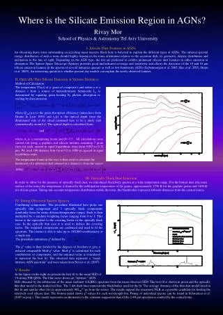
Explore the intriguing silicate dust features in Active Galactic Nuclei (AGNs) through modeling and fitting techniques. Discover the role of torus orientation, geometry, and density in the infrared emission spectrum. Utilize Spitzer Space Telescope data to detect and analyze silicate emission features in different AGN types.

E N D
I. Silicate Dust Features in AGNs An obscuring dusty torus surrounding an accreting super massive black hole is believed to explain the different types of AGNs. The infrared spectral energy distribution of such a torus should highly depend on the torus orientation relative to the accretion disk, its geometry, density distribution and inclination to the line of sight. Depending on the AGN type, the tori are predicted to exhibit prominent silicate dust features in either emission or absorption. The Spitzer Space Telescope (Spitzer) provides good mid-infrared coverage and sensitivity and allows the detection of the 10 and 18 μm silicate emission features in the spectra of several luminous quasars as well as low-luminosity AGNs (Siebenmorgen et al. 2005; Hao et al. 2005; Strum et al. 2005). An interesting question is whether present day models can explain the newly observed features. Where is the Silicate Emission Region in AGNs? II. Optically Thin Silicate Emission at Various Distances Method of Calculation: The temperature Ti(a,r) of a grain of composite i and radius a at a distance r from a source of monochromatic luminosity Lυ is determined by equating grain heating by photon absorption to cooling by dust emission: where Qiabs(a,υ) is the grain absorption efficiency (taken here from Draine & Laor 1993) and τυ(r) is the optical depth from the illuminated side of the cloud (assumed here to be a dusty slab symmetrically around r). The optical depth is calculated from: and where Ai is a normalizing factor and β=-3.5 . All calculations were carried out using a graphite and silicate mixture assuming 7 grain sizes for each, spaced in equal logarithmic steps from 0.005 to 0.32 μm. We used 100 distance bins from 0.2 to 1000 pc spaced in equal logarithmic steps. The temperature found in this way is then used to calculate the luminosity of a spherical shell situated at a distance r from the source using: Rivay Mor School of Physics & Astronomy Tel Aviv University III. Optically Thick Dust Emission In order to allow for the presence of optically thick dust, we introduced blackbody spectra at a wide temperature range. For the hottest dust (the inner surface of the torus) the temperature is limited by the sublimation temperature of the grains, approximately 1750 K for the graphite grains and 1400 K for silicate grains. Taking into account temperature distribution within the torus, the blackbodies represent different distances from the central source. IV. Fitting Observed Spitzer Spectra Combining components: The procedure illustrated here picks one optically thin component and 3 optically thick components (randomly from the entire distance/temperature range). Each is then multiplied by a random weighting factor ranging from 0 to 1. This factor is the equivalent to the covering factor in the optically thick case. In the optically thin case it is used to deduce the covering factor. The weighted components are combined and used to fit the spectrum. The routine is able to take up to 100,000 combinations at a single run. The procedure minimizes χ2 defined by: The χ2 value is then divided by the degrees of freedom to give a reduced comparable Mod-χ2 value. Mod-χ2 is calculated for each combination of components, and the minimal value is considered to represent the best fit. The observed data represent a “mean intrinsic AGN spectrum” and were taken from Netzer et al. (2007). V. Results In the figure on the right we present the best fit to the mean SED of 10 strong FIR QSOs. The blue curve shows an “intrinsic” AGN SED obtained by the subtraction of the mean starburst (ULIRG) spectrum from the mean observed SED. The best fit is shown in green and the optically thin dust model is the dashed red line. The 3 dot-dash lines represent the blackbodies used for the fit. The average distance of the thin dust model (used in this fit and similar other fits) is approximately 90L460.5 pc from the source. The results support the innermost NLR as a possible candidate for hosting the relatively cool silicate dust. The bottom panel shows χ2 values for each wavelength bin. Fitting of individual spectra can be found in Schweitzer et al. (2007 in prep.). This model represents an alternative to the common suggestion that all the 2-40 μm spectrum is emitted by the central torus.