Download

1 / 44
440 likes | 520 Views
Wissensverarbeitung - Search -. Alexander Felfernig und Gerald Steinbauer Institut für Softwaretechnologie Inffeldgasse 16b/2 A-8010 Graz Austria. Skriptum (TU Wien, Institut für Informationssysteme, Thomas Eiter et al.) ÖH- Copyshop , Studienzentrum

E N D
Wissensverarbeitung- Search - Alexander Felfernig und Gerald Steinbauer Institut für Softwaretechnologie Inffeldgasse 16b/2 A-8010 Graz Austria
Skriptum (TU Wien, Institut für Informationssysteme, Thomas Eiter et al.) ÖH-Copyshop, Studienzentrum Stuart Russell und Peter Norvig. ArtificialIntelligence - A Modern Approach. Prentice Hall. 2003. Vorlesungsfolien TU Graz (partiallybased on theslidesofTUWien) References
Uninformed Search Strategies. Informed Search Strategies. Goals
ImportantmethodofArtificialIntelligence Approaches: Uninformedsearch Informedsearch (exploitinformation/heuristicsabouttheproblemstructure) Example: Whichistheshortestpathfrom A to D? Search D A B C E
Start node (startstate) Goal node (goalstate) States aregenerateddynamically on thebasisofgenerationrule R example: moveoneelementtotheemptyfield Searchgoal: sequenceofrulesthattransformthestartstatetothegoalstate Elements of a Search Problem 3 6 1 2 3 start state goal state 2 1 4 8 4 5 8 7 7 6 5
Start state (S0) Non-empty set of goal states (goal test) Non-empty set of operators: Transform state Si into state Si+1 Transformation triggers costs (>0) No cost estimation available default: unit costs Cost function for search paths: of individual transformations Search Problem
Completeness Does the method find a solution, if one exists? Space Complexity How do memory requirements increase with increasing sizes of search problems (search spaces)? Time Complexity What is the computing performance with increasing sizes of search problems (search spaces)? Optimality Does the method identify the optimal solution (if one exists)? Properties of Search Methods
Level-wise expansion of states Systematic strategy Expand all paths of length 1 Expand all paths of length 2 … Completeness yes (if b is finite). Space complexity: branching factor b, depth of the shallowest solution d: bd+1 Time complexity: bd+1 Optimality yes (if step costs are identical). Breadth-First Search (bfs)
[A] … [B,C,D] [B,C,D] … [C,D,E,F] [C,D,E,F] … [D,E,F,G] [D,E,F,G] … [E,F,G] [E,F,G] … [F,G] [F,G] … [G] [G] bfs D G F A C B E
Goal: „cheapest“ path from S to G (independent of # transitions) Approach: Expand S, then expand A (since A has the cheapest current path) Solution not necessarily found opt. could be < 11 Expand B finally solution identified with path costs = 10 Uniform Cost Search (ucs) A S 10 1 A B C 5 5 G S B S 1 5 15 S 5 15 A B C A B C C 15 15 5 G A G 11 10 11
Generalization of bfs Expand state with lowest related costs There could be a solution with shorter path but higher costs Corresponds to bfsif step costs are identical Completeness yes (if b finite & step costs > ). Space complexity: branching factor b, cost of the optimal solution C*: bC*/ + 1 Time complexity: bC*/ + 1 Optimality yes. Uniform Cost Search (ucs)
No level-wise expansion Expansion of successor nodes of one „deepest state“ If no more states can be expanded backtracking Completeness no (indefinite descent paths) Space complexity: branching factor b, maximum depth of the search tree m: bm Time complexity: bm Optimality no. Depth First Search (dfs)
[A] … [B,C,D] [B,C,D] … [E,F,C,D] [E,F,C,D] … [H,F,C,D] [H,F,C,D] … [F,C,D] [F,C,D] … [C,D] [C,D] … [F,G,D] [F,G,D] … [G,D] [G,D] dfs D G F A C B E H
Searchdepthdefinedbyboundl Ifsearchdepthlisreached backtracking Ifnosolutionhasbeenfoundforlevell l = l + 1 Exampleusing a binarytree: Level 0: Level 1: Level 2: DF Iterative Deepening (dfid) Repeateddfs untilsearchlevell.
Completeness yes (if b is finite). Space complexity: branching factor b, depth of the shallowest solution d: bd Time complexity: bd Optimality yes (if step costs are identical). DF Iterative Deepening
Informed search which exploits problem- and domain-specific knowledge Estimation function: estimates the costs from the current node to the goal state Heuristic approach denoted as best-first search, since best-evaluated state is chosen for expansion Used notation: f: estimation function; f* (the real function) h(n): estimator of minimal costs from n to a goal state Invariant for goal state Sn: h(n) = 0 Methods to be discussed: Greedy search A* search Heuristic Search
Estimates minimal costs from current to the goal node Does not take into account already existing costs, i.e., f(n) = h(n) Completeness no (loopcheck needed). Space complexity: branching factor b, maximum depth of the search tree m : bm Time complexity: bm Optimality no. Greedy Search
Greedy Search straight-line distance – h(sld)
Greedy Search straight-line distance – h(sld)
Greedy Search straight-line distance – h(sld)
Use sld heuristics Choose shortest path from Arad to Bucharest Arad: expand lowest h-value Sibiu: expand lowest h-value Fagaras: expand lowest h-value Bucharest found path: Arad, Sibiu, Rimnicu, Pitesti, Bucharest length of solution: 418km (in contrast to solution found – 450km) Greedy search is based on local information Better choice: take into account already existing “efforts” Summarizing Greedy Search
In contrast to greedy search, it takes into account already existing costs as well. g(n) = path costs from start to current node Results in a more fair selecting strategy for expansion Estimation function: f(n) = g(n) + h(n); h(n) the same as for greedy search A*: best-first search method with the following properties: Finite number of possible expansions Transition costs are positive (min. ) admissible (h), i.e., h does never overestimate the real costs (it is an optimistic heuristic) Consequently: fnever overestimates the real costs A* Search
Usedfunctions g(n): real distanceArad-n h(n): sldBucharest-n Takingintoaccount global informationimprovesthequalityoftheidentifiedsolution Expansion ordering (lowestf-value) Sibiu, Rimnicu, Pitesti, Bucharest Optimal solution will befound Summarizing A* Search
Heuristic function h must be optimistic No formal rule set of determining heuristic functions exists, however, some rules of thumb are there … Example (8-Puzzle) 2 heuristic functions h1 and h2 h1: number of squares in wrong position h2: sum(distances of fields from goal state) Simplification: do not take into account the influences of moves to other fields. For start state, h1=7 and h2 = 15 Dominance relationship: h2 dominates h1 since for each n: h1(n) h2(n) h2 is assumed to be more efficient; h1 has tendency towards breadth first search. Determination of Heuristics start state goal state
f-values along a path in the search tree are never decreasing (monotonicity property) theorem: monoton(f) h(n1) c(n1,n2) + h(n2) expansion of nodes with increasing f-value Properties of A* Search goal
„Distance circles“ of 380, 400, 420km (f-values) Expand all n with f(n)380, then 400, … Let f* be the costs of an optimal solution: A* expands all n with f(n) < f* , some m with f(m) = f*, and the goal state will be identified Completeness yes (h is admissible). Space complexity: exponential Time complexity: exponential Optimality yes. Properties of A* Search
Optimality of A* Search Suppose suboptimal goal (path to) G2 in the queue. Let n be an unexpanded node on a shortest path to an optimal goal G f(G2 ) = g(G2 ) since h(G2 )=0 > g(G) since G2 is suboptimal [f(G2) > g(G)] • >= f(n) since h is admissible [f(G2) > f(n)] Since f(G2) > f(n), A* will never select G2 for expansion
Previously: systematic exploration of search space path to goal is solution to the problem However, for some problems the path is irrelevant for example, 8-queens problem state space = set of configurations (complete) goal: identify configuration which satisfies a set of constraints Other algorithms can be used local search algorithms try to improve the current state by generating a follow-up state (neighbor state) are not systematic, not optimal, and not complete Local Search
n-queens problem: positioning of n queens in an nxn board s.t. the number of 2 queens positioned on the same column, row or diagonal is minimized or zero. Local Search: Example
“Finding the top of Mount Everest in a thick fog while suffering from amnesia” [Russel & Norvig, 2003] “Greedy local search” Hill Climbing Algorithm
Peak that is higher than each of its neighboring states but lower than the global maximum. Hill Climbing: Local Maxima • h = number of pairs of queens attacking each other • successor function: move single queen to another square in the same column • h = 1 • local maximum (minimum): “every move of a single queen makes the situation worse” • [Russel & Norvig 2003]
Sequence of local maxima. Hill Climbing: Ridges
Evaluation function is “flat”, a local maximum or a shoulder from which progress is possible. Hill Climbing: Plateaux
Hill climbing never selects downhill moves Danger of, for example, local maxima Instead of picking the best move, choose a random one and accept also worse solutions with a decreasing probability Simulated Annealing
Start with k randomly generated states (the population) Each state (individual) represented by a string over a finite alphabet (e.g., 1..8) Each state is rated by evaluation (fitness) function (e.g., #non-attacking pairs of queens – opt. = 28) Selection probability directly proportional to fitness score, for example, 23/(24+23+20+11) 29% Genetic Algorithms
Genetic Algorithm function GENETIC_ALGORITHM( population, FITNESS-FN) return an individual input:population, a set of individuals FITNESS-FN, a function which determines the quality of the individual repeat new_population empty set loop forifrom 1 to SIZE(population) do x RANDOM_SELECTION(population, FITNESS_FN) y RANDOM_SELECTION(population, FITNESS_FN) child REPRODUCE(x,y) if (small random probability) then child MUTATE(child ) add child to new_population population new_population until some individual is fit enough or enough time has elapsed return the best individual