Understanding Automated Planning and Decision Making: Concepts and Search Algorithms
This overview discusses the foundations of automated planning and decision-making, emphasizing the nature of search problems, search spaces, and goal conditions. It delves into examples like the Rubik's Cube and the n-Queens problem, illustrating critical concepts such as states, operators, and goal conditions. The description of search methods, including blind and informed search strategies, highlights their significance in navigating vast solution spaces. This comprehensive guide provides insight into how search algorithms influence problem-solving efficiency in artificial intelligence.


Understanding Automated Planning and Decision Making: Concepts and Search Algorithms
E N D
Presentation Transcript
Search Automated Planning and Decision Making Prof. Ronen Brafman Automated Planning and Decision Making 2007 1
Introduction • In the past, most problems you encountered were such that the way to solve them was very “clear” and straight forward: • Solving quadratic equation. • Solving linear equation. • Matching input to a regular expression • Most of the problems in AI are of different kind. • NP-Hard problems. • Require searching in a large solution space. Automated Planning and Decision Making 2
Search Problem • A set S of possible states – the search space. • Initial State: sI in S. • Operators - which take us from one state to another (S→S functions) • Goal Conditions. Automated Planning and Decision Making 3
The Search Space • A graph G(V,E) where: • V={v : v in S} • E={<v,u> : exists o in Operators such that o(v)=u} 4
The Task • Find a path in the search space from sI to a state s where the Goal Conditions are valid. • Sometimes we only care about s, and not the path • Sometimes we only care whether s exists. • Sometimes value is associated with states, and we want the best s. • Sometimes cost is associated with operators, and we want the cheapest path
Search Problem Example • Finding a solution for Rubik's Cube. • SI: Some state of the cube. • Operators: 90o rotation of any of the 9 plates. • Goal Conditions: same color for each of the cube's sides. • The Search Space will include: • A node for any possible state of the cube. • An edge between two nodes if you can reach from one to the other by a 90o rotation of some plate. Automated Planning and Decision Making 4
Another Example • States: Locations of Tiles. • Operators: Move blank right/left/down/up. • Goal Conditions: As in the picture. • Note: optimal solution of n-Puzzle family isNP-hard… Initial State Goal State Automated Planning and Decision Making 5
Example: n queens problem(a constraint satisfaction problem) States: legal placements of k≤n queens Operators: add a queen Goal condition: n queens placed with no conflicts (no constraint violated)
Example: n queens problemAn alternative formulation States: placements of n queens – one per column Operators: move one of the queens Goal condition: n queens placed with no conflicts (no constraint violated)
Solving Search Problems • Apply the Operators on States in order to expand (produce) new States, until we find one that satisfies the Goal Conditions. • At any moment we may have different options to proceed (multiple Operators may apply) • Q: In what order should we expand the States? • Our choice affects: • Computation time • Space used • Whether we reach an optimal solution • Whether we are guaranteed to find a solution if one exists (completeness) Automated Planning and Decision Making 6
Search Tree • You can think of the search as spanning a tree: • Root: The initial state. • Children of node v are all states reachable from v by applying an operator. • We can reach the same state via different paths. • In such a case, we can ignore this duplicate state, and treat it as a leaf node • Requires that we remember all states we visited! • Important parameters affecting performance: • b – Average branching factor. • d – Depth of the closest solution. • m – Maximal depth of the tree. • Fringe: set of current leaf (unexpanded) nodes Automated Planning and Decision Making 7
Search Methods • Different search methods differ in the order in which they visit/expand the nodes. • It is important to distinguish between: • The search space • The order by which we scan that space • These are orthogonal issues! • Some algorithms are described abstractly by describing the space they generate w/o specifying how it is searched • You can implement them in different ways by choosing different search algorithms • Blind Search • No additional information about search states is used. • Informed Search • Additional information used to improve search efficiency Automated Planning and Decision Making 8
Relation to Planning • Simplest (and currently most popular) way to solve planning problem is to search from the initial state to a goal • Search states are states of the world • Operators = actions • There are other formulations! • For instance: search states = plans • Search is a very general technique – very important for many applications beyond planning Automated Planning and Decision Making 9
Blind Search Automated Planning and Decision Making 10
Blind Search • Main algorithms: • DFS – Depth First Search • Expand the deepest unexpanded node. • Fringe is a LIFO. • BFS – Breath First Search • Expand the shallowest unexpanded node. • Fringe is a FIFO. • IDS – Iterative Deepening Search • Combines the advantages of both methods. • Avoids the disadvantages of each method. • There many are other variants (e.g., optimizing disk access, parallel search, etc.) Automated Planning and Decision Making 11
1 4 2 3 Breadth First Search Automated Planning and Decision Making 12
Properties of BFS • Complete?Yes (if b is finite). • Time?1+b+b2+b3+…+b(bd-1)=O(bd+1( • Space? O(bd) (keeps every node on the fringe). • Optimal?Yes (if cost is 1 per step). • Space is a BIG problem… Automated Planning and Decision Making 13
10 11 12 5 6 7 8 9 1 2 3 4 Depth First Search Automated Planning and Decision Making 14
Properties of DFS • Complete? • No if given infinite branches (e.g., when we have loops) • Easy to modify: check for repeat states along path • Complete in finite spaces! • May require large space to maintain list of visited states • Time? • Worst case: O(bm). • Terrible if m is much larger then d. • But if solutions occur often or in the “left” part of the tree, may be much faster then BFS. • Space? • O(m) Linear Space! • Optimal? • No. Automated Planning and Decision Making 15
Depth Limited Search • DFS with a depth limit ℓ, i.e., nodes at depth ℓ have no successors. Automated Planning and Decision Making 16
Iterative Deepening Search • Increase the depth limit of the DLS with each Iteration: Automated Planning and Decision Making 17
Complexity of IDS • Number of nodes generated in a depth-limited search to depth d with branching factor b: NDLS = b0 + b1 + b2 + … + bd-2 + bd-1 + bd • Number of nodes generated in an iterative deepening search to depth d with branching factor b: NIDS = (d+1)b0 + db1 + (d-1)b2 + … + 3bd-2 +2bd-1 + 1bd • For b = 10, d = 5: • NDLS = 1 + 10 + 100 + 1,000 + 10,000 + 100,000 = 111,111 • NIDS= 6 + 50 + 400 + 3,000 + 20,000 + 100,000 = 123,456 • Overhead = (123,456 - 111,111)/111,111 = 11% Automated Planning and Decision Making 19
Properties of IDS • Complete?Yes. • Time?(d+1)b0 + db1 + (d-1)b2 + … + bd = O(bd) • Space?O(d) • Optimal?Yes. If step cost is 1. Automated Planning and Decision Making 20
Comparison of the Algorithms Automated Planning and Decision Making 21
General Search Scheme • Solve(Nodes) • if empty Nodes -> return Failure • else • let Node = Select-Node(Nodes) • let Rest = Nodes - Node • if Node is Goal -> return Solution • else • let Children = Expand-Node(Node) • let New-Nodes = Add-Nodes(Children, Nodes) • Solve(New-Nodes) • Different algorithms obtained by suitable instantiation of Select-Node and Add-Nodes • Nodes are data structures that contain state and bookkeeping info • Initially Nodes = {root}
Some Blind Instances of GSS • DFS expands “deepest” node first • Select-Node: select first Node in Nodes • Add-Nodes: Puts Children before Nodes • Implementation: Nodes is a stack (LIFO) • Breadth-First Search expands ’shallowest’ nodes first • Select-Node: select first Node in Nodes • Add-Nodes: Puts Children after Nodes • Implementation: Nodes is a queue (FIFO)
Bounded GSS • Solve(Nodes,Bound) • if empty Nodes -> return Failure • else • let Node = Select-Node(Nodes) • let Rest = Nodes - Node • if f(Node) > Bound • Solve(Rest, Bound) ;;; PRUNE Node • else if Node is Goal -> return ProcessSolution(Node,Rest) • else • let Children = Expand-Node(Node) • let New-Nodes = Add-Nodes(Children, Nodes) • Solve(New-Nodes,Bound) • IDS calls Bounded GSS with bound 1,2,3,... • ProcessSolution(Node,Rest) returns Node as solution
Bidirectional Search • Assumptions: • There is a small number of states satisfying the goal conditions. • It is possible to reverse the operators. • Simultaneously run BFS from both directions. • Stop when reaching a state from both directions. • Under the assumption that validating this overlap takes constant time, we get: • Time: O(bd/2) • Space: O(bd/2) Automated Planning and Decision Making 22
Informed Search Automated Planning and Decision Making 23
Informed/Heuristic Search • Heuristic Function h:S→R • For every state s, h(s) is an estimation of the minimal distance/cost from s to a solution. • Distance is only one way to set a price. • How to produce h? later on… • Cost Function g:S→R • For every state s, g(s) is the minimal cost to s from the initial state. • f=g+h, is an estimation of the cost from the initial state to a solution. Automated Planning and Decision Making 24
Properties of Heuristics • h is perfect if h(s) = shortest distance to goal from s (and ∞if goal is unreachable from s) • The perfect heuristic is denoted by h* • h is safe if h(s)=∞ implies h*(s)=∞ • h is goal-aware if h(s)=0 for every goal state s • h is admissible if h(s)≤h*(s) for all s • h is consistent if h(s)≤h(s’)+1 whenever s’ is a child of s
Best First Search • Greedy on h values. • Fringe stored in a queue ordered by h values. • In every step, expand the “best” node so far, i.e., the one with the best h value. Automated Planning and Decision Making 25
Properties of Best First • Complete? • No, can get into loops • Yes, with duplicate detection and safe h • Time? • O(bm). But a good heuristic can give dramatic improvement. • Space? • O(bm). Keeps all nodes in memory. • Optimal • No. Automated Planning and Decision Making 28
A* Search • Idea: Avoid expanding paths that are already expensive. • Greedy on f values. • Fringe is stored in a queue ordered by f values. • Recall, f(n)=g(n)+h(n), where: • g(n): cost so far to reach n. • h(n): estimated cost from n to goal. • f(n): estimated total cost of path through n to goal. Automated Planning and Decision Making 29
Slides 5-12 41
Admissible Heuristics • A heuristic h(n) is admissible if for every node n, h(n) ≤ h*(n), where h*(n) is the realcost to reach the goal state from n. • An admissible heuristic never overestimates the cost to reach the goal, i.e., it is optimistic • Theorem:If h(n) is admissible, A* using Tree-Search is optimal. • Tree search – nodes encountered more than once are not treated as leaf nodes Automated Planning and Decision Making 32
Optimality of A* (Proof) • Suppose some suboptimal goal G2 has been generated and is in the fringe. Let n be an unexpanded node in the fringe such that n is on a shortest path to an optimal goal G. Automated Planning and Decision Making 33
Optimality of A* (Proof) • f(G2) = g(G2) since h(G2) = 0. • f(G) = g(G) since h(G) = 0. • g(G2) > g(G) since G2 is suboptimal. • f(G2) > f(G) by 1,2,3. • h(n) ≤ h*(n) since h is admissible. • g(n)+h(n) ≤ g(n)+h*(n) by 5. • f(n) ≤ f(G) by definition of f. • f(G2) > f(n) by 4,7. Hence A* will never select G2 for expansion. Automated Planning and Decision Making 34
Properties of A* • Complete? • Yes, unless there are infinitely many nodes with f ≤ f(G). • Time? • Exponential. • Optimal? • Yes. • Space? • Keeps all nodes in memory. • A serious problem in many cases! • How can we overcome it? Automated Planning and Decision Making 37
Iterative Deepening A* (IDA*) • Combine Iterative Deepening with A* in order to overcome the space problem. • A simple idea: • Replace upper bound on depth with upper bound on f values. • If f(n)>U, n is not enqueued. • If no solution is found given U, increase U. • Another method -- Weighted A* (soon) Automated Planning and Decision Making 38
Branch & Bound • Used for finding an optimal solution (i.e., when there are multiple possible solutions, but some are better than others) • Attempts to prune entire sub-trees • Applicable in the context of different search methods (BFS, DFS, …). • Assumes we can generate upper bound U and lower bound L on the value of solutions reachable from n • If for some node n there exists a node n’ such that U(n)<I(n’), we can prune n. • Often used as follows: • First, quickly find any solution with value v’ • Prune any node n s.t. f(n) > v’ Automated Planning and Decision Making 39