Download
1 / 20
200 likes | 289 Views
4. Closed - Loop Responses Using the Laplace Transform Method. 4.1 The Laplace Transform. The Laplace transform allows algebraic manipulation of ordinary differential equations (ODE’s). Solution of ODE’s is difficult, so, Transform the problem to a domain, where the solution is easier.

E N D
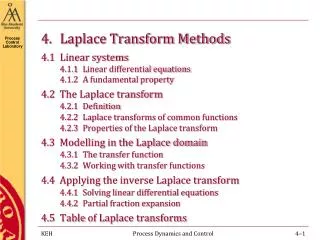
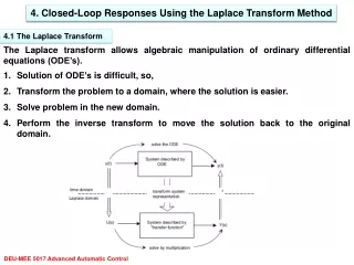
4. Closed-LoopResponsesUsing the Laplace TransformMethod 4.1 The Laplace Transform The Laplace transform allows algebraic manipulation of ordinary differential equations (ODE’s). • Solution of ODE’s is difficult, so, • Transform the problem to a domain, where the solution is easier. • Solve problem in the new domain. • Perform the inverse transform to move the solution back to the original domain. DEU-MEE 5017 Advanced Automatic Control
Definition: 4.2 SomeCommonExamplesUsed in Control Theory Unit step function: Exponential function: Impulse function:
4.3 MajorProperties of Laplace Transform • Delaying f(t) by a delay time equals to multiplying its transform F(s) by e-s . • Remember that f(t) starts at t=0 and f(t- ) starts at t= .
Example 4.1: Find the transfer function from ODE of a system Transfer function of a system is the ratio of the Laplace transform of output to the Laplace transform of input when the initial conditions are zero. • A fundemental assumption when using the transfer function to compute responses is that the system is at rest at time t=0. • The differentiating property can be used to find the transfer function of a system that is at rest at time t=0.
4.2 The Inverse Laplace Transform Laplace transform Inverse Laplace transform Tables can be used for Laplace and inverse transforms.
Let eigenvalues of systems be in the fom of If (real poles) Then, Inverse transform If (complex poles) Then, Inverse transform
4.3 PartialFractionExpansion (Heaviside’sMethod) Laplace transform of outputs can be expressed as a sum of partial fraction to be able to take the inverse transfrom. Heaviside method systematically converts a polynomial quatient . Heaviside method is used to find the unkonown coefficients (Ai, i=1,2,…n) in the numerator. Pi, i=1,2,…m are the eigenavalues, which are real or complex constants. If eigenvalues have real poles, then the coefficients of Ai have real values. If eigenvalues have complex poles, then the coefficients of Ai have complex values. 4.3a.Distinctpoles: The method applies only to the case of distinct poles of the denominator. (It is called as cover-up method )
4.3b. Repeatedpoles: The method applies only to the case of repeated poles of the denominator. If p1, p2,p3,…pm are the repeated poles, then C(s) can be written a sum of partial fractions. . . .
Example 4.2: Find the time response of the output C(s) byusinginversetransform. Eigenvalues for closed loop system: p1=-3, p2=-1, p3=-1, p4=0 Partial fraction expansion: are determined by Heaviside method.
Check the results of Heaviside’s method by MATLAB code: nvs=[1-1];dvs=[1 5 7 3 0];[r,p,k]=residue(nvs,dvs)
MATLAB code to plot time response: t=0:dt:ts; vsan= 1/3*exp(-3*t) + t.*exp(-t) - 1/3; plot(t,vsan,'or') Verify the response by MATLAB/Simulink.
Example 4.3a Find step response of Example 3.1 by Laplace solution PI control (Kp=6, Ki=2) Eigenvalues for closed loop system: p1,2=-0.33±0.3018i VR(t) = 10 (Step input) Partial fraction expansion:
p1,2=-0.33±0.3018i are determined by Heaviside method Check the results of Heaviside’s method by MATLAB code: nvs=10*[0.6 0.2];dvs=[1 0.66 0.2 0];[r,p,k]=residue(nvs,dvs)
The result of partial fraction expansion of C(s) Im 8.9455i Re -10.
MATLAB code to plot time response: t=0:dt:ts; vsan=13.4172*exp(-0.33*t).*cos(0.3018*t-2.4118)+10; plot(t,vsan,'or') Verify the response by MATLAB/Simulink.
Example 4.3bSolveExample 3.1with a time delay by the Laplace method. PI control (Kp=6, Ki=2, td=12 s) VR(t) = 10 u(t-td), step input with a delay td clc;clear;close all td=12; nh=10*[0.6 0.2];dh=[1 0.66 0.2]; h=tf(nh,dh,'InputDelay',td),step(h) % Step response by Laplace transform [r,p,k]=residue(nh,[dh 0]) p0=p(1);cksi_v2;z=2*r(2);a=abs(z);fi=angle(z); sigma=abs(real(p(1)));w=abs(imag(p(1))); t=0:dt:ts;c=a*exp(-sigma*t).*cos(w*t-fi)+r(3); hold on;plot(td+t,c,'--r')
Example 4.4 SolveExample 3.2 by the Laplace method. for P control (Kp=400) x2(t) =? r(t) = 0.1 (Step input)
iω ωn φ -σ 4.4 Evaluating Eigenvalues 4.4a Eigenvalues havecomplexpoles : p=-σ+iω Im fn=1/Tn Re Responses for second order systems Undamped natural frequency (rad/s) Damped natural frequency) (rad/s) Undamped periyot (s) Undamped natural frequency (Hz) Damping ratio Time step (s) Settling time (s)
4.4b Eigenvalues haverealpoles : p=-σ Responses for first order systems Time constant (s) Time step (s) Settling time (s)