Laplace Transform
Laplace Transform. Melissa Meagher Meagan Pitluck Nathan Cutler Matt Abernethy Thomas Noel Scott Drotar. The French Newton Pierre-Simon Laplace. Developed mathematics in astronomy, physics, and statistics Began work in calculus which led to the Laplace Transform


Laplace Transform
E N D
Presentation Transcript
Laplace Transform Melissa Meagher Meagan Pitluck Nathan Cutler Matt Abernethy Thomas Noel Scott Drotar
The French NewtonPierre-Simon Laplace • Developed mathematics in astronomy, physics, and statistics • Began work in calculus which led to the Laplace Transform • Focused later on celestial mechanics • One of the first scientists to suggest the existence of black holes
History of the Transform • Euler began looking at integrals as solutions to differential equations in the mid 1700’s: • Lagrange took this a step further while working on probability density functions and looked at forms of the following equation: • Finally, in 1785, Laplace began using a transformation to solve equations of finite differences which eventually lead to the current transform
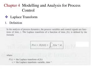
Definition • The Laplace transform is a linear operator that switched a function f(t) to F(s). • Specifically: where: • Go from time argument with real input to a complex angular frequency input which is complex.
Restrictions • There are two governing factors that determine whether Laplace transforms can be used: • f(t) must be at least piecewise continuous for t ≥ 0 • |f(t)| ≤ Meγt where M and γ are constants
Continuity • Since the general form of the Laplace transform is: it makes sense that f(t) must be at least piecewise continuous for t ≥ 0. • If f(t) were very nasty, the integral would not be computable.
Boundedness • This criterion also follows directly from the general definition: • If f(t) is not bounded by Meγt then the integral will not converge.
Laplace Transform Theory • General Theory • Example • Convergence
Laplace Transforms • Some Laplace Transforms • Wide variety of function can be transformed • Inverse Transform • Often requires partial fractions or other manipulation to find a form that is easy to apply the inverse
Laplace Transform for ODEs • Equation with initial conditions • Laplace transform is linear • Apply derivative formula • Rearrange • Take the inverse
Laplace Transform in PDEs Laplace transform in two variables (always taken with respect to time variable, t): Inverse laplace of a 2 dimensional PDE: Can be used for any dimension PDE: The Transform reduces dimension by “1”: • ODEs reduce to algebraic equations • PDEs reduce to either an ODE (if original equation dimension 2) or another PDE (if original equation dimension >2)
Consider the case where: ux+ut=t with u(x,0)=0 and u(0,t)=t2 and Taking the Laplace of the initial equation leaves Ux+ U=1/s2 (note that the partials with respect to “x” do not disappear) with boundary condition U(0,s)=2/s3 Solving this as an ODE of variable x, U(x,s)=c(s)e-x + 1/s2 Plugging in B.C., 2/s3=c(s) + 1/s2 so c(s)=2/s3 - 1/s2 U(x,s)=(2/s3 - 1/s2) e-x + 1/s2 Now, we can use the inverse Laplace Transform with respect to s to find u(x,t)=t2e-x - te-x + t
Diffusion Equation ut = kuxx in (0,l) Initial Conditions: u(0,t) = u(l,t) = 1, u(x,0) = 1 + sin(πx/l) Using af(t) + bg(t) aF(s) + bG(s) and df/dt sF(s) – f(0) and noting that the partials with respect to x commute with the transforms with respect to t, the Laplace transform U(x,s) satisfies sU(x,s) – u(x,0) = kUxx(x,s) With eat 1/(s-a) and a=0, the boundary conditions become U(0,s) = U(l,s) = 1/s. So we have an ODE in the variable x together with some boundary conditions. The solution is then: U(x,s) = 1/s + (1/(s+kπ2/l2))sin(πx/l) Therefore, when we invert the transform, using the Laplace table: u(x,t) = 1 + e-kπ2t/l2sin(πx/l)
Wave Equation utt = c2uxx in 0 < x < ∞ Initial Conditions: u(0,t) = f(t), u(x,0) = ut(x,0) = 0 For x ∞, we assume that u(x,t) 0. Because the initial conditions vanish, the Laplace transform satisfies s2U = c2Uxx U(0,s) = F(s) Solving this ODE, we get U(x,s) = a(s)e-sx/c + b(s)esx/c Where a(s) and b(s) are to be determined. From the assumed property of u, we expect that U(x,s) 0 as x ∞. Therefore, b(s) = 0. Hence, U(x,s) = F(s) e-sx/c. Now we use H(t-b)f(t-b) e-bsF(s) To get u(x,t) = H(t – x/c)f(t – x/c).
Real-Life Applications Semiconductor mobility Call completion in wireless networks Vehicle vibrations on compressed rails Behavior of magnetic and electric fields above the atmosphere
Ex. Semiconductor Mobility • Motivation • semiconductors are commonly made with superlattices having layers of differing compositions • need to determine properties of carriers in each layer • concentration of electrons and holes • mobility of electrons and holes • conductivity tensor can be related to Laplace transform of electron and hole densities
Notation R = ratio of induced electric field to the product of the current density and the applied magnetic field ρ = electrical resistance H = magnetic field J = current density E = applied electric field n = concentration of electrons u = mobility
Assuming a continuous mobility distribution and that , , it follows:
Source Johnson, William B. Transform method for semiconductor mobility, Journal of Applied Physics 99 (2006).