Download
1 / 26
270 likes | 455 Views
If your several predictors are categorical , MRA is identical to ANOVA. If your sole predictor is continuous , MRA is identical to correlational analysis. If your sole predictor is dichotomous , MRA is identical to a t-test. Do your residuals meet the required assumptions ?.

E N D
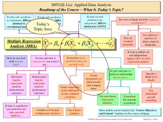
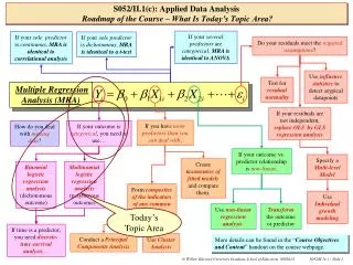
If your several predictors are categorical, MRA is identical to ANOVA If your sole predictor is continuous, MRA is identical to correlational analysis If your solepredictor is dichotomous, MRA is identical to a t-test Do your residuals meet the required assumptions? Use influence statistics to detect atypical datapoints Test for residual normality Multiple Regression Analysis (MRA) If your residuals are not independent, replace OLS byGLS regression analysis If you have more predictors than you can deal with, If your outcome is categorical, you need to use… If your outcome vs. predictor relationship isnon-linear, Specify a Multi-level Model Create taxonomies of fitted models and compare them. Binomiallogistic regression analysis (dichotomous outcome) Multinomial logistic regression analysis (polytomous outcome) Discriminant Analysis Form composites of the indicators of any common construct. Use Individual growth modeling Today’s Topic Area Transform the outcome or predictor Use non-linear regression analysis. If time is a predictor, you need discrete-time survival analysis… Conduct a Principal Components Analysis Use Cluster Analysis S052/II.2(b): Applied Data AnalysisRoadmap of the Course – What Is Today’s Topic Area? More details can be found in the “Course Objectives and Content” handout on the course webpage.
Today, I will: • Introduce the multinomial logistic regression model, distinguishing it from the binomial logistic regression model. • Fit a taxonomy of multinomial logistic regression models. • Compare and contrast the output obtained in a multinomial and a binomial logit analysis. • Explain an additional test (“Type III Analysis of Effects”) that is available in a multinomial logit analysis. • Test and interpret a fitted multinomial logistic regression model. S052/II.2(b): Extensions of the Basic Logit Approach/Multinomial Logit AnalysisPrinted Syllabus – What Is Today’s Topic? Please check inter-connections among the Roadmap, the Daily Topic Area, the Printed Syllabus, and the content of today’s class when you pre-read the day’s materials.
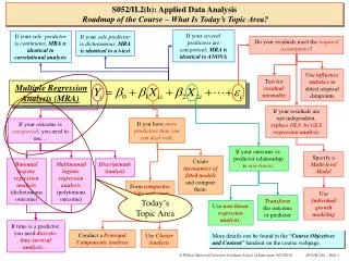
Broad Research Question: How is entry into college impacted by race/ethnicity and socio-economic status? Radcliffe, Class of ‘57 S052/II.2(b): Extensions of the Basic Logit Approach/Multinomial Logit AnalysisIntroducing the Alternative Routes to Education Dataset Information accompanying today’s dataset is in ALT_RTS_GIRLS_info.pdf….
Polychotomous categorical outcome variable Principle question predictors S052/II.2(b): Extensions of the Basic Logit Approach/Multinomial Logit AnalysisPrinted Syllabus – What Is Today’s Topic?
We still use the logistic regression function, containing usual parameters and predictors, to represent right hand side of the model But, because the outcome is no longer a dichotomy, we have to do something about the left-hand side of the model. P(Comm Coll vs. No Coll) 1 • Under the multinomial logit approach, we simultaneously model the relationship between predictors and twooutcome probabilities: • Probability of going to community college vs. not going to college, • Probability of going to 4-year college vs. not going to college. 0 SES 1 P(4-Year vs. No Coll) S052/II.2(b): Extensions of the Basic Logit Approach/Multinomial Logit AnalysisHow Do You Model The Relationship Between A Polytomous Outcome & Predictors? To model the relationship between a polychotomous outcome, like COLLEGE (which has three categories – “Four-Year College,” “Community College,” & “No College”) and a predictor like SES, we use the same “logit” approach that we have already developed …
S052/II.2(b): Extensions of the Basic Logit Approach/Multinomial Logit AnalysisHow Do You Model The Relationship Between A Polytomous Outcome & Predictors? So, the hypothesized multinomial logit model simply becomes a simultaneous collection of two parts … Both parts of the new multinomial model are fitted simultaneously to the data, with parameter estimates and goodness-of-fit statistics interpreted in the usual way …
Standard input statements Create a categorical variable representing race/ethnicity for use in subsequent tabulations Creates a set of two-way interactions needed in subsequent logistic regression analyses. Format selected categorical variables for use in subsequent tabulations S052/II.2(b): Extensions of the Basic Logit Approach/Multinomial Logit AnalysisReading The Alternative Routes Data Into PC-SAS Data-Analytic Handout II_2b_1… *---------------------------------------------------------------------------------* Input the data, name and label the variables in the dataset *---------------------------------------------------------------------------------*; DATA ALT_RTS_GIRLS; INFILE 'C:\DATA\S052\ALT_RTS_GIRLS.txt'; INPUT ID COLLEGE HSGRAD READ MATH WHITE BLACK LATINO SES; LABEL COLLEGE = 'Institution Selected for Postsec Ed' BLACK = 'Is respondent African-American?' LATINO = 'Is respondent Hispanic?' WHITE = 'Is respondent Caucasian?‘ SES = 'Socio-economic status'; * Create a single categorical variable to represent race/ethnicity; IF BLACK=1 THEN RACE=1; IF LATINO=1 THEN RACE=2; IF WHITE=1 THEN RACE=3; * Create the required two-way interactions between RACE and SES; BxSES = BLACK*SES; LxSES = LATINO*SES; WxSES = WHITE*SES; PROC FORMAT; VALUE CFMT 1='No Postsec Ed' 2='Tech/Voc or Comm Coll' 3='4-Year College'; VALUE RFMT 1='Black' 2='Latino' 3='White';
Compute the 2 statistic Eliminate row percentages Compute the cell contributions to the 2 statistic Standard two-way contingency-table analysis of the bivariate relationship between categorical variables COLLEGE and RACE. Obtaining descriptive statistics on continuous variable SES within each of the COLLEGE by RACE subgroups (this is useful for subsequent plotting of prototypical fitted trend lines). Compute statistics by RACE, and for ALL the sample. Estimate the 5th %ile, median and 95th %ile of SES for each group S052/II.2(b): Extensions of the Basic Logit Approach/Multinomial Logit AnalysisProgramming Exploratory Data Analysis In The Alternative Routes Dataset First, let’s conduct exploratory analyses to examine the bivariate relationships between the polychotomous outcomeCOLLEGE and predictors RACE and SES using classical contingency table analysis … *---------------------------------------------------------------------------------* Obtaining statistics on COLLEGE choice for the different racial/ethnic groups *---------------------------------------------------------------------------------*; * Cross-tabulation of COLLEGE and RACE; PROC FREQ DATA=ALT_RTS_GIRLS; TABLE COLLEGE*RACE / NOROW CHISQ CELLCHI2; FORMAT RACE RFMT. COLLEGE CFMT.; * Distribution of SES by COLLEGE and RACE; PROC TABULATE DATA=ALT_RTS_GIRLS; CLASS COLLEGE RACE; VAR SES; TABLE (COLLEGE*(RACE ALL)),(SES*(P5 MEDIAN P95)); FORMAT RACE RFMT. COLLEGE CFMT.;
Standard test associated with a two-way contingency analysis: • The sample 2 statistic compares the observed frequencies to the frequencies expected under the null hypothesis. • The statistic is computed as follows: H0:COLLEGE and RACE are not related, in the population. Test statistic & p-value:2 = 112.75 ( p<.0001) Decision: Reject H0 Conclusion: In the population, race/ethnicity is an important predictor of a girl’s choice of type of college. S052/II.2(b): Extensions of the Basic Logit Approach/Multinomial Logit AnalysisClassical Contingency Table Analysis In The Alternative Routes Dataset COLLEGE(Institution Selected for Postsec Ed) RACE Frequency ‚ Cell Chi-Square ‚ Percent ‚ Col Pct ‚Black ‚Latino ‚White ‚ Total ƒƒƒƒƒƒƒƒƒƒƒƒƒƒƒƒƒˆƒƒƒƒƒƒƒƒˆƒƒƒƒƒƒƒƒˆƒƒƒƒƒƒƒƒˆ No Postsec Ed ‚ 120 ‚ 192 ‚ 716 ‚ 1028 ‚ 1.1294 ‚ 16.74 ‚ 4.6433 ‚ ‚ 2.21 ‚ 3.54 ‚ 13.22 ‚ 18.97 ‚ 20.91 ‚ 25.46 ‚ 17.51 ‚ ƒƒƒƒƒƒƒƒƒƒƒƒƒƒƒƒƒˆƒƒƒƒƒƒƒƒˆƒƒƒƒƒƒƒƒˆƒƒƒƒƒƒƒƒˆ Tech/Voc or Comm ‚ 225 ‚ 365 ‚ 1467 ‚ 2057 Coll ‚ 0.2297 ‚ 21.656 ‚ 4.7421 ‚ ‚ 4.15 ‚ 6.74 ‚ 27.08 ‚ 37.97 ‚ 39.20 ‚ 48.41 ‚ 35.87 ‚ ƒƒƒƒƒƒƒƒƒƒƒƒƒƒƒƒƒˆƒƒƒƒƒƒƒƒˆƒƒƒƒƒƒƒƒˆƒƒƒƒƒƒƒƒˆ 4-Year College ‚ 229 ‚ 197 ‚ 1907 ‚ 2333 ‚ 1.3351 ‚ 50.206 ‚ 12.077 ‚ ‚ 4.23 ‚ 3.64 ‚ 35.20 ‚ 43.06 ‚ 39.90 ‚ 26.13 ‚ 46.63 ‚ ƒƒƒƒƒƒƒƒƒƒƒƒƒƒƒƒƒˆƒƒƒƒƒƒƒƒˆƒƒƒƒƒƒƒƒˆƒƒƒƒƒƒƒƒˆ Total 574 754 4090 5418 10.59 13.92 75.49 100.00 Statistics for Table of COLLEGE by RACE Statistic DF Value Prob ƒƒƒƒƒƒƒƒƒƒƒƒƒƒƒƒƒƒƒƒƒƒƒƒƒƒƒƒƒƒƒƒƒƒƒƒƒƒƒƒƒƒƒƒƒƒƒƒƒƒƒƒƒƒ Chi-Square 4 112.7585 <.0001 Likelihood Ratio Chi-Square 4 117.5525 <.0001 Mantel-Haenszel Chi-Square 1 41.2598 <.0001
A useful diagnostic tool that can help you determine where the detected relationship really resides…. • Examine each cell for a “large” contribution to the 2 statistic: • The story is really about Latinos: • More Latinos than expected are going to community college, or not going to college at all. • Fewer Latinos than expected are going to 4 year college. • However, there are a few more Whites than expected going to 4-year college. S052/II.2(b): Extensions of the Basic Logit Approach/Multinomial Logit AnalysisClassical Contingency Table Analysis In The Alternative Routes Dataset COLLEGE(Institution Selected for Postsec Ed) RACE Frequency ‚ Cell Chi-Square ‚ Percent ‚ Col Pct ‚Black ‚Latino ‚White ‚ Total ƒƒƒƒƒƒƒƒƒƒƒƒƒƒƒƒƒˆƒƒƒƒƒƒƒƒˆƒƒƒƒƒƒƒƒˆƒƒƒƒƒƒƒƒˆ No Postsec Ed ‚ 120 ‚ 192 ‚ 716 ‚ 1028 ‚ 1.1294 ‚ 16.74 ‚ 4.6433 ‚ ‚ 2.21 ‚ 3.54 ‚ 13.22 ‚ 18.97 ‚ 20.91 ‚ 25.46 ‚ 17.51 ‚ ƒƒƒƒƒƒƒƒƒƒƒƒƒƒƒƒƒˆƒƒƒƒƒƒƒƒˆƒƒƒƒƒƒƒƒˆƒƒƒƒƒƒƒƒˆ Tech/Voc or Comm ‚ 225 ‚ 365 ‚ 1467 ‚ 2057 Coll ‚ 0.2297 ‚ 21.656 ‚ 4.7421 ‚ ‚ 4.15 ‚ 6.74 ‚ 27.08 ‚ 37.97 ‚ 39.20 ‚ 48.41 ‚ 35.87 ‚ ƒƒƒƒƒƒƒƒƒƒƒƒƒƒƒƒƒˆƒƒƒƒƒƒƒƒˆƒƒƒƒƒƒƒƒˆƒƒƒƒƒƒƒƒˆ 4-Year College ‚ 229 ‚ 197 ‚ 1907 ‚ 2333 ‚ 1.3351 ‚ 50.206 ‚ 12.077 ‚ ‚ 4.23 ‚ 3.64 ‚ 35.20 ‚ 43.06 ‚ 39.90 ‚ 26.13 ‚ 46.63 ‚ ƒƒƒƒƒƒƒƒƒƒƒƒƒƒƒƒƒˆƒƒƒƒƒƒƒƒˆƒƒƒƒƒƒƒƒˆƒƒƒƒƒƒƒƒˆ Total 574 754 4090 5418 10.59 13.92 75.49 100.00 Statistics for Table of COLLEGE by RACE Statistic DF Value Prob ƒƒƒƒƒƒƒƒƒƒƒƒƒƒƒƒƒƒƒƒƒƒƒƒƒƒƒƒƒƒƒƒƒƒƒƒƒƒƒƒƒƒƒƒƒƒƒƒƒƒƒƒƒƒ Chi-Square 4 112.7585 <.0001 Likelihood Ratio Chi-Square 4 117.5525 <.0001 Mantel-Haenszel Chi-Square 1 41.2598 <.0001
Useful to know, when we produce prototypical fitted plots…. S052/II.2(b): Extensions of the Basic Logit Approach/Multinomial Logit AnalysisTabulation of SES, by COLLEGE and RACE „ƒƒƒƒƒƒƒƒƒƒƒƒƒƒƒƒƒƒƒ…ƒƒƒƒƒƒƒƒƒƒƒƒƒƒƒƒƒƒƒƒƒƒƒƒƒƒƒƒƒƒƒƒƒƒƒƒƒƒ† ‚‚ Socio-economic status ‚ ‚ ‡ƒƒƒƒƒƒƒƒƒƒƒƒ…ƒƒƒƒƒƒƒƒƒƒƒƒ…ƒƒƒƒƒƒƒƒƒƒƒƒ‰ ‚ ‚ P5 ‚ Median ‚ P95 ‚ ‡ƒƒƒƒƒƒƒƒƒ…ƒƒƒƒƒƒƒƒƒˆƒƒƒƒƒƒƒƒƒƒƒƒˆƒƒƒƒƒƒƒƒƒƒƒƒˆƒƒƒƒƒƒƒƒƒƒƒƒ‰ ‚Institut-‚RACE ‚ ‚ ‚ ‚ ‚ion ‚ ‚ ‚ ‚ ‚ ‚Selected ‚ ‚ ‚ ‚ ‚ ‚for ‚ ‚ ‚ ‚ ‚ ‚Postsec ‚ ‚ ‚ ‚ ‚ ‚Ed ‚ ‚ ‚ ‚ ‚ ‡ƒƒƒƒƒƒƒƒƒˆƒƒƒƒƒƒƒƒƒ‰ ‚ ‚ ‚ ‚No ‚Black ‚ 0.99‚ 1.96‚ 3.19‚ ‚Postsec ‡ƒƒƒƒƒƒƒƒƒˆƒƒƒƒƒƒƒƒƒƒƒƒˆƒƒƒƒƒƒƒƒƒƒƒƒˆƒƒƒƒƒƒƒƒƒƒƒƒ‰ ‚Ed ‚Latino ‚ 1.06‚ 1.81‚ 2.99‚ ‚ ‡ƒƒƒƒƒƒƒƒƒˆƒƒƒƒƒƒƒƒƒƒƒƒˆƒƒƒƒƒƒƒƒƒƒƒƒˆƒƒƒƒƒƒƒƒƒƒƒƒ‰ ‚ ‚White ‚ 1.45‚ 2.38‚ 3.42‚ ‚ ‡ƒƒƒƒƒƒƒƒƒˆƒƒƒƒƒƒƒƒƒƒƒƒˆƒƒƒƒƒƒƒƒƒƒƒƒˆƒƒƒƒƒƒƒƒƒƒƒƒ‰ ‚ ‚All ‚ 1.34‚ 2.28‚ 3.34‚ ‡ƒƒƒƒƒƒƒƒƒˆƒƒƒƒƒƒƒƒƒˆƒƒƒƒƒƒƒƒƒƒƒƒˆƒƒƒƒƒƒƒƒƒƒƒƒˆƒƒƒƒƒƒƒƒƒƒƒƒ‰ ‚Tech/Voc ‚RACE ‚ ‚ ‚ ‚ ‚or Comm ‡ƒƒƒƒƒƒƒƒƒ‰ ‚ ‚ ‚ ‚Coll ‚Black ‚ 1.30‚ 2.41‚ 3.55‚ ‚ ‡ƒƒƒƒƒƒƒƒƒˆƒƒƒƒƒƒƒƒƒƒƒƒˆƒƒƒƒƒƒƒƒƒƒƒƒˆƒƒƒƒƒƒƒƒƒƒƒƒ‰ ‚ ‚Latino ‚ 1.42‚ 2.33‚ 3.68‚ ‚ ‡ƒƒƒƒƒƒƒƒƒˆƒƒƒƒƒƒƒƒƒƒƒƒˆƒƒƒƒƒƒƒƒƒƒƒƒˆƒƒƒƒƒƒƒƒƒƒƒƒ‰ ‚ ‚White ‚ 1.79‚ 2.84‚ 3.81‚ ‚ ‡ƒƒƒƒƒƒƒƒƒˆƒƒƒƒƒƒƒƒƒƒƒƒˆƒƒƒƒƒƒƒƒƒƒƒƒˆƒƒƒƒƒƒƒƒƒƒƒƒ‰ ‚ ‚All ‚ 1.62‚ 2.74‚ 3.76‚ ‡ƒƒƒƒƒƒƒƒƒˆƒƒƒƒƒƒƒƒƒˆƒƒƒƒƒƒƒƒƒƒƒƒˆƒƒƒƒƒƒƒƒƒƒƒƒˆƒƒƒƒƒƒƒƒƒƒƒƒ‰ ‚4-Year ‚RACE ‚ ‚ ‚ ‚ ‚College ‡ƒƒƒƒƒƒƒƒƒ‰ ‚ ‚ ‚ ‚ ‚Black ‚ 1.63‚ 2.98‚ 4.15‚ ‚ ‡ƒƒƒƒƒƒƒƒƒˆƒƒƒƒƒƒƒƒƒƒƒƒˆƒƒƒƒƒƒƒƒƒƒƒƒˆƒƒƒƒƒƒƒƒƒƒƒƒ‰ ‚ ‚Latino ‚ 1.49‚ 2.68‚ 4.13‚ ‚ ‡ƒƒƒƒƒƒƒƒƒˆƒƒƒƒƒƒƒƒƒƒƒƒˆƒƒƒƒƒƒƒƒƒƒƒƒˆƒƒƒƒƒƒƒƒƒƒƒƒ‰ ‚ ‚White ‚ 2.20‚ 3.37‚ 4.39‚ ‚ ‡ƒƒƒƒƒƒƒƒƒˆƒƒƒƒƒƒƒƒƒƒƒƒˆƒƒƒƒƒƒƒƒƒƒƒƒˆƒƒƒƒƒƒƒƒƒƒƒƒ‰ ‚ ‚All ‚ 1.97‚ 3.28‚ 4.36‚ Šƒƒƒƒƒƒƒƒƒ‹ƒƒƒƒƒƒƒƒƒ‹ƒƒƒƒƒƒƒƒƒƒƒƒ‹ƒƒƒƒƒƒƒƒƒƒƒƒ‹ƒƒƒƒƒƒƒƒƒƒƒƒŒ
When fitting a multinomial model, you must specify the common reference category that will be used in each of the simultaneous binomial comparisons: • Here, I have chosen “1” or “no college” as the reference category. • Any of the available categories can be selected – it’s a substantive choice, not a statistical one. • PROCLOGISTIC can fit models for several categorical outcomes: • Binomial logit (by default, if the outcome is dichotomous), • Ordinal logit (by default, if the outcome is ordinal and more than two categories), • Multinomial logit, if you choose the GLOGIT (“generalized logit”) “link” function. S052/II.2(b): Extensions of the Basic Logit Approach/Multinomial Logit AnalysisFitting A Taxonomy of Multinomial Logit Models To The Alternative Routes Data *---------------------------------------------------------------------------------* Fitting A Taxonomy Of Nested Multinomial Logit Models *---------------------------------------------------------------------------------*; PROC LOGISTIC DATA=ALT_RTS_GIRLS; M1: MODEL COLLEGE(ref='1')= BLACK LATINO / LINK=GLOGIT EXPB RSQUARE; PROC LOGISTIC DATA=ALT_RTS_GIRLS; M2: MODEL COLLEGE(ref='1')= SES / LINK=GLOGIT EXPB RSQUARE; PROC LOGISTIC DATA=ALT_RTS_GIRLS; M3: MODEL COLLEGE(ref='1')= BLACK LATINO SES / LINK=GLOGIT EXPB RSQUARE; PROC LOGISTIC DATA=ALT_RTS_GIRLS; M4: MODEL COLLEGE(ref='1')= BLACK LATINO SES BxSES LxSES / LINK=GLOGIT EXPB RSQUARE;
Confirms that a multinomial logit model has been fitted Tells you thatthree levelshave been detected in the outcome variable. Confirms that the “no college” option (COLLEGE=1) is being used as the reference category. S052/II.2(b): Extensions of the Basic Logit Approach/Multinomial Logit Analysis1st Page Of Output For Any Model Confirms That A Multinomial Logit Model Has Been Fit Examine the output for Model M1, containing the main effects of only predictors BLACK and LATINO … The LOGISTIC Procedure Model Information Data Set WORK.ALT_RTS_GIRLS Response Variable COLLEGE Institution Selected for Postsec Ed Number of Response Levels 3 Number of Observations 5418 Model generalized logit Optimization Technique Fisher's scoring Response Profile Ordered Total Value COLLEGE Frequency 1 1 1028 2 2 2057 3 3 2333 Logits modeled use COLLEGE=1 as the reference category. Model Convergence Status Convergence criterion (GCONV=1E-8) satisfied. The history of the fitting process looks very similar to that produced in regular logistic regression analysis, but contains interesting distinguishing information
H0: The simultaneous effect of all predictors in Model M1 (race predictors, BLACK and LATINO) on a girl’s choice of college is zero, in the population. Test Statistic: 2 = 117.55 (df=4), p< .0001 Decision: Reject H0 Conclusion: In the population, a girl’s college choice depends on her race. S052/II.2(b): Extensions of the Basic Logit Approach/Multinomial Logit AnalysisOverall Fit Of The Model Is Assessed In The Usual WayBy The -2LL Statistic Model Fit Statistics Intercept Intercept and Criterion Only Covariates -2 Log L 11333.060 11215.508 R-Square 0.0215 Max-rescaled R-Square 0.0245 Testing Global Null Hypothesis: BETA=0 Test Chi-Square DF Pr > ChiSq Likelihood Ratio 117.5525 4 <.0001
All parameter estimates are present in pairs because there were two outcome comparisons • Under “COLLEGE” is recorded the label of the “upper” category: • “2” represents community college, • “3” represents 4-year college. There are two sets of parameter estimates, one for each facet of the multinomial model: S052/II.2(b): Extensions of the Basic Logit Approach/Multinomial Logit AnalysisParameter Estimates, And Ancillary Statistics, Are Present To Excess Analysis of Maximum Likelihood Estimates Standard Wald Parameter COLLEGE DF Estimate Error Chi-Square Pr > ChiSq Exp(Est) Intercept 2 1 0.7173 0.0456 247.5623 <.0001 2.049 Intercept 3 1 0.9796 0.0438 499.5382 <.0001 2.663 BLACK 2 1 -0.0887 0.1219 0.5294 0.4668 0.915 BLACK 3 1 -0.3334 0.1209 7.6013 0.0058 0.717 LATINO 2 1 -0.0749 0.1001 0.5594 0.4545 0.928 LATINO 3 1 -0.9539 0.1105 74.5501 <.0001 0.385
Both these confidence intervals cover unity (the “null” value for an odds-ratio), and so: • We cannot reject the null hypothesis in either case. • There are no statistically significant differences in the probability of going to community college/vocational training (e.g., outcome = 2) among girls of all three race/ethnicities. When odds-ratios are less than unity, it’s best to invert them, for interpretive purposes, but remember to invert the interpretation too The fitted odds that a Caucasian girl will go to Four-Year College (vs. not going to college at all) is 1.39 times the fitted odds that an African –American girl will have the same outcome. “The fitted odds that a Caucasian girl will go to Four-Year college (vs. choosing no college at all) is 2.6 times the fitted odds that a Latino girl will have the same outcome” S052/II.2(b): Extensions of the Basic Logit Approach/Multinomial Logit AnalysisAntilogged Parameter Estimates Are Also Provided, To Be Interpreted As Odds-Ratios Odds Ratio Estimates Point 95% Wald Effect COLLEGE Estimate Confidence Limits BLACK 2 0.915 0.721 1.162 BLACK 3 0.717 0.565 0.908 LATINO 2 0.928 0.763 1.129 LATINO 3 0.385 0.310 0.478
Test statistic: difference in –2LL 2 = (9901.5-9864.7) = 36.8 Critical value: 2(df=4;=.05) = 9.49 Decision: Reject H0 Conclusion: Controlling for the main effects of race/ethnicity and socioeconomic status, the post-secondary education choices of African-American, Latina and Caucasian girls depend on their socioeconomic status, in the population. S052/II.2(b): Extensions of the Basic Logit Approach/Multinomial Logit AnalysisFinal Taxonomy Of Fitted Multinomial Logit Models Taxonomy of fitted multinomial logit models of the relationship between a girl’s choice of postsecondary institution and her race/ethnicity and socioeconomic status (n=5148). Key: ~ p<.10; * p<.05; ** p<.01; *** p<.001
Test Statistic: 2 = 6.43, df=2, p=0.04 Decision: Reject H0 Conclusion: Postsecondary education choices of Black and White girls differ by their SES, in the population. S052/II.2(b): Extensions of the Basic Logit Approach/Multinomial Logit AnalysisThere Are Additional “Type III” Tests,If You Want To Test The Impact Of A Single Predictor On The Joint Outcome Taxonomy of fitted multinomial logit models of the relationship between a girl’s choice of postsecondary institution and her race/ethnicity and socioeconomic status (n=5148). Type III Analysis of Effects Wald Effect DF Chi-Square Pr > ChiSq BLACK 2 12.4539 0.0020 LATINO 2 29.8929 <.0001 SES 2 789.6798 <.0001 BxSES 2 6.4279 0.0402 LxSES 2 36.1789 <.0001 Key: ~ p<.10; * p<.05; ** p<.01; *** p<.001
Test Statistics: 2 = 36.18 (df=2), p<.0001 Decision: Reject H0 Conclusion: Postsecondary education choices of Latina and White girls differ by their SES, in the population. S052/II.2(b): Extensions of the Basic Logit Approach/Multinomial Logit AnalysisThere Are Additional “Type III” Tests,If You Want To Test The Impact Of A Single Predictor On The Joint Outcome Taxonomy of fitted multinomial logit models of the relationship between a girl’s choice of postsecondary institution and her race/ethnicity and socioeconomic status (n=5148). Type III Analysis of Effects Wald Effect DF Chi-Square Pr > ChiSq BLACK 2 12.4539 0.0020 LATINO 2 29.8929 <.0001 SES 2 789.6798 <.0001 BxSES 2 6.4279 0.0402 LxSES 2 36.1789 <.0001 Key: ~ p<.10; * p<.05; ** p<.01; *** p<.001
S052/II.2(b): Extensions of the Basic Logit Approach/Multinomial Logit AnalysisWriting Down Fitted Models Is Straightforward We can recover prototypical fitted equations in the usual way…but, now there are two sets …
S052/II.2(b): Extensions of the Basic Logit Approach/Multinomial Logit AnalysisProducing Fitted Plots For Prototypical Individuals Is Just The Same 4-Year College vs. No College Community College vs. No College L B B Among female adolescents who do not go to community college: • High SES youth are more likely to go to 4-yr college than low SES youth, and these differences are greater than corresponding effects for enrollment in community college. • At low SES, all youth have a lower probability of going to four-year college than to community college, but B & L youth have a similar and higher probability of enrolling in a 4-yr college than W youth. • At high SES, B & W youth have a similar and higher probability of enrolling in a four-year college than do L youth. L W W • Among female adolescents who do not go to four-year college: • High SES youth are more likely to enroll in community college than low SES youth. • At each level of SES, with an effect larger at low SES, B & L youth have a similar and higher probability of enrolling in community college than W youth.
S052/II.2(b): Extensions of the Basic Logit Approach/Multinomial Logit AnalysisAppendix I: An Algebraic Aside On The Inversion Of Odds-ratios Odds-ratios can be inverted, you just have to get the interpretation correct …
Create a pair of new dichotomous outcomes: • COMCOLL indicates whether the student went to community college, • FOURYR indicates whether the student went to a four-year college. Comparison group is the “no postsecondary education” group, in each case Use contingency-table analysis to examine the relationship between the two new dichotomous outcomes, COMCOLL and FOURYR S052/II.2(b): Extensions of the Basic Logit Approach/Multinomial Logit AnalysisAppendix II: Does Using Multinomial Logistic Regression Have AdvantagesOver Using Multiple Binomial Logistic Regressions? A comparison of results obtained when fitting a multinomial logit versus a pair of binomial logit models to the same data can be found in Data-Analytic Handout II_2b_2 … *--------------------------------------------------------------------------------* Input the data, name and label the variables in the dataset *--------------------------------------------------------------------------------*; DATA ALT_RTS_GIRLS; INFILE 'C:\DATA\S052\ALT_RTS_GIRLS.txt'; INPUT ID COLLEGE HSGRAD READ MATH WHITE BLACK LATINO SES; LABEL COLLEGE = 'Institution Selected for Postsec Ed' BLACK = 'Is respondent African-American?' LATINO = 'Is respondent Hispanic?' WHITE = 'Is respondent Caucasian?' SES = 'Socio-economic status'; * Create the required two-way interactions between RACE and SES; BxSES = BLACK*SES; LxSES = LATINO*SES; * Create a pair of new dichotomous outcomes to replace polytomous COLLEGE; IF COLLEGE=2 THEN COMCOLL=1; ELSE COMCOLL=0; IF COLLEGE=3 THEN FOURYR=1; ELSE FOURYR=0; * Format the new outcomes; PROC FORMAT; VALUE CCFMT 0='No Postsec Ed' 1='Tech/Voc or Comm Coll'; VALUE FYFMT 0='No Postsec Ed' 1='4-Year College'; *-------------------------------------------------------------------------------- Are the New Binomial Outcomes Independent? *--------------------------------------------------------------------------------; PROC FREQ DATA=ALT_RTS_GIRLS; FORMAT COMCOLL CCFMT. FOURYR FYFMT.; TABLES COMCOLL*FOURYR /CHISQ;
Same baseline group appears in both binomial comparisons. Empty cell. Reject H0 and conclude that COMCOLL and FOURYR are not independent, in the population. The phi coefficient is equivalent to a Pearson’s correlation coefficient, for a pair of dichotomous variables: r = -0.63 So, we conclude that the two new dichtomous outcomes are strongly correleated S052/II.2(b): Extensions of the Basic Logit Approach/Multinomial Logit AnalysisAppendix II: Does Using Multinomial Logistic Regression Have AdvantagesOver Using Multiple Binomial Logistic Regressions? Notice the interesting relationship between the two newly-created dichotomous outcomes … Table of COMCOLL by FOURYR COMCOLL FOURYR Frequency ‚ Percent ‚ Row Pct ‚ Col Pct ‚No Posts‚4-Year C‚ Total ‚ec Ed ‚ollege ‚ ƒƒƒƒƒƒƒƒƒƒƒƒƒƒƒƒƒˆƒƒƒƒƒƒƒƒˆƒƒƒƒƒƒƒƒˆ No Postsec Ed ‚ 1028 ‚ 2333 ‚ 3361 ‚ 18.97 ‚ 43.06 ‚ 62.03 ‚ 30.59 ‚ 69.41 ‚ ‚ 33.32 ‚ 100.00 ‚ ƒƒƒƒƒƒƒƒƒƒƒƒƒƒƒƒƒˆƒƒƒƒƒƒƒƒˆƒƒƒƒƒƒƒƒˆ Tech/Voc or Comm ‚ 2057 ‚ 0 ‚ 2057 Coll ‚ 37.97 ‚ 0.00 ‚ 37.97 ‚ 100.00 ‚ 0.00 ‚ ‚ 66.68 ‚ 0.00 ‚ ƒƒƒƒƒƒƒƒƒƒƒƒƒƒƒƒƒˆƒƒƒƒƒƒƒƒˆƒƒƒƒƒƒƒƒˆ Total 3085 2333 5418 56.94 43.06 100.00 Statistics for Table of COMCOLL by FOURYR Statistic DF Value Prob ƒƒƒƒƒƒƒƒƒƒƒƒƒƒƒƒƒƒƒƒƒƒƒƒƒƒƒƒƒƒƒƒƒƒƒƒƒƒƒƒƒƒƒƒƒƒƒƒƒƒƒƒƒƒ Chi-Square 1 2507.6352 <.0001 Likelihood Ratio Chi-Square 1 3267.1645 <.0001 Continuity Adj. Chi-Square 1 2504.8049 <.0001 Mantel-Haenszel Chi-Square 1 2507.1723 <.0001 Phi Coefficient -0.6803
Two separate binomial logistic regression analyses: • COMCOLL vs no postsecondary education. • FOURYR vs no postsecondary education. S052/II.2(b): Extensions of the Basic Logit Approach/Multinomial Logit AnalysisAppendix II: Does Using Multinomial Logistic Regression Have AdvantagesOver Using Multiple Binomial Logistic Regressions? *--------------------------------------------------------------------------------* Fit a binomial logit model for the community college vs. no postsec comparison; *--------------------------------------------------------------------------------*; * Pick out the sub-sample for the community college vs. no postsec comparison; DATA ALT_RTS_GIRLS_COMCOLL; SET ALT_RTS_GIRLS; IF COLLEGE NE 3; * Fit the associated binomial logit model; PROC LOGISTIC DATA=ALT_RTS_GIRLS_COMCOLL; M4A: MODEL COMCOLL(event='1')= BLACK LATINO SES BxSES LxSES; *---------------------------------------------------------------------------------* Fit the binomial logit model for the four-year college vs. no postsec comparison; *--------------------------------------------------------------------------------*; * Pick out the sub-sample for the four year vs. no postsec comparison; DATA ALT_RTS_GIRLS_FOURYR; SET ALT_RTS_GIRLS; IF COLLEGE NE 2; * Fit the associated binomial logit model; PROC LOGISTIC DATA=ALT_RTS_GIRLS_FOURYR; M4B: MODEL FOURYR(event='1')= BLACK LATINO SES BxSES LxSES;
Different samples are employed in the multinomial and the twin binomial approaches. The parameter estimates arenot particularly affected in any systematic way -- some estimates are higher for one outcome, some higher for the other. Sample size is the largest in the multinomial analysis. So, the standard errors are always smaller in the multinomial analysis. S052/II.2(b): Extensions of the Basic Logit Approach/Multinomial Logit AnalysisAppendix II: Does Using Multinomial Logistic Regression Have AdvantagesOver Using Multiple Binomial Logistic Regressions?