Download
1 / 60
600 likes | 726 Views
Approaches to Continental Scale River Flow Routing. by Kwabena Oduro Asante Dr David Maidment Dr James Famiglietti Dr Francisco Olivera Dr Randall Charbeneau Dr Daene McKinney. Acknowledgements. Dissertation Committee National Science Foundation EROS Data Center of the USGS

E N D
Approaches toContinental Scale River Flow Routing by Kwabena Oduro Asante Dr David Maidment Dr James Famiglietti Dr Francisco Olivera Dr Randall Charbeneau Dr Daene McKinney
Acknowledgements Dissertation Committee National Science Foundation EROS Data Center of the USGS GIS Hydro Research Group Global Hydrology Group
Dissertation Outline • Chapter 1: General Introduction • Chapter 2: Literature Review • Chapter 3: Data Development • Chapter 4: STS and HMS Methodology • Chapter 5: Model Applications • Chapter 6: Conclusions and Recommendations
Motivation • The changing scope of hydrologic problems • Local scale to global scale • Single phase to full hydrologic cycle • Spatially lumped to spatially distributed • The limitations of current routing models • Local scale models untested at global scale • Lack of integration of hydrologic cycle phases • Scale dependence of existing large scale models
Objectives • To develop adatabase of hydrologic parameters to support continental scale runoff routing • To implement a continental scale runoff routing system for transferring water balance model outputs to ocean models • To examine the robustness of the modeling approach implemented as compared to a watershed based approach
Conceptual Models of a River Basin Cell-to-Cell CTC Watershed Based HMS Source-to-Sink STS
S = KQ Q t Q = I * f(k,n) Q = I * f(v,D) I I Q Q I Q s s s s Methods of Characterizing Flow Translation with Incidental Dispersion Example: Linear Reservoir Routing I Q S Translation with Surrogate Dispersion Example: Cascade of Linear Reservoirs Translation with Physically Based Dispersion Example: Diffusion Wave Routing I Q
Chapter 3:Data Development Study Objective 1 “to develop a GIS database to support large-scale surface water routing globally”
Terrain Analysis Identify Inland Catchments and insert in projected DEM Fill DEM and Compute Flow Direction Lower Datum and Project DEM Delineate Drainage Basins Compute Flow Length Compute Flow Accumulation
GIS Hydro ‘99:Digital Atlas Digital Atlas of the World Water Balance www.crwr.utexas.edu
2 Preprocessing for theSource to sink (STS) model 1 Delineate Drainage Basins from Sink Locations Define Sinks along continental margin and within Inland Catchments 3 4 Define Sources while preserving basin boundaries as well as Ocean and Atmospheric modeling units Determine routing parameters for each Source from Flow length and other Spatially distributed data
Linking to Ocean and WaterBalance Models STS Modeling Units
2 1 Preprocessing for the Hydrologic Modeling System (HMS) Delineate Watersheds from outlet grid and Flow direction grid and convert to a vector coverage Delineate Stream Network from Flow Accumulation Grid and define outlets at stream intersections 3 4 Create HMS basin file detailing element properties and connectivity Compute stream and watershed parameters and connectivity
Chapter 4:Methodology Study Objective 2 “to implement a modeling framework which incorporates basin boundaries in a grid based model while maintaining computational efficiency by only performing routing at desired locations”
STS Modeling Assumptions • The control volume is the flow path from a given source to its sink • The transfer of flow along the flow path is a linear process • The parameters of the transfer function are time invariant
Listing of source properties and their connectivity to sinks and to other models Parameters such as no. of events, outlets, sources and routing interval FORTRAN code for Routing with and without dispersion Input runoff files and output files containing the results of simulation runs Sinks listed by sink id STS Model Components
Diffusion Wave IRF V = velocity in m/s D = disp. coef. in m2/s P = 3.14159….. x = distance in m t = time in s
Input Runoff from GCM (generated by Branstetter,M.)
HMS Modeling Assumptions • Each hydrologic element has a unique control volume linked to the next downstream element • The transfer of flow along the flow path may be linear or non-linear • The parameters of the transfer function are time invariant
Simulation parameters such as start and end time and interval Routing Codes for methods assigned in the basin file Description of input runoff and relation to basin elements Listing of properties of hydrologic elements and their connectivity Data Storage System including input runoff and routed flow data HMS Model Components
HMS Flow Routing Subbasin Response by SCS Unit Hydrograph with lag_time = max { (0.6 maxlagtime in minutes), 3.5 interval} River Reach Response by Muskingum Routing with n = int (2 x K / 60) + 1 Numerical stability Pure Translation
Chapter 5:Model Applications Study Objective 3 “to examine of the robustness of the source to sink approach as compared to the watershed based approach in continental scale applications”
The Application Basins The Congo Basin Area = 3.78 million km2 Mean flow = 45 000 m3/s The Nile Basin Area =3.25 million km2 Mean flow = 2,500 m3/s
STS Model Runs STS Model of the Nile Basin STS Model of the Congo Basin
Longitudinal Decomposability in STS 1000 km 1200 km 800 km 2000 km
! Longitudinal Decomposability in STS Cell 4 Cell 3 Cell 2 Cell 1
Effect of STS Modeling Unit Size Source size = 30’ (60 x 60 km) Source size = 10’ (20 x 20 km) Source size = 5’ (10 x 10 km)
Effect of Spatial Resolution STS basin response for the Congo • !
Effect of Temporal Resolution STS basin response for the Congo • !
Effect of Spatial Distribution of V and D on STS basin response for the Nile
Effect of Spatial Distribution of Velocity STS basin response for the Nile Distributed V is important !
Effect of Spatial Distribution of Dispersion STS basin response for the Nile Distributed D is not critical !
Combined Effect of Velocity and Dispersion STS basin response for the Nile Distributed V and D is best !
HMS Model Runs The Nile Basin The Congo Basin
Longitudinal Decomposability in HMS reach length = 162,000 m flow velocity = 0.3 m/s muskingum K = 0.3 n = 4 n = 5 n = 6 n = 7 n = 8
Longitudinal Decomposability in HMS higher n = less dispersion !
Effect of HMS Modeling Unit Size Stream Delineation Threshold of 10,000 km2 Stream Delineation Threshold of 1,000 km2
Effect of Spatial Resolution HMS Basin Response for the Congo HMS is spatially scale dependent !
Effect of Temporal Resolution on HMS Congo Basin Response Higher routing interval = more dispersion
ComparingSTS and HMS Basin Responses STS Model of the Congo Basin HMS Model of the Congo Basin
Comparing STS and HMS Basin Responses Congo Basin, 1000 km2 threshold responses almost identical !
Comparing STS and HMS Basin Responses Congo Basin, 10000 km2 threshold responses at higher threshold not identical !
Comparing STS and HMS Basin Responses Nile Basin, Spatially Distributed V and D
Comparing STS and HMS Basin Responses for Non-uniform Velocity Case, Nile Basin Similar responses result from a common grid of V and D !
Comparing Simulated Flows with Observed Data