Download
1 / 19
360 likes | 2.03k Views
Hydrologic River Flood Routing. Basic Equation. Muskingum Method. For a non-uniform flow , S t f(O t ) Because I t =f(y 1 ) and O t = f(y 2 ) . Therefore, S t =f(I t ,O t ) . Prism storage = f(O t ); Wedge storage = f(I t , O t ).

E N D
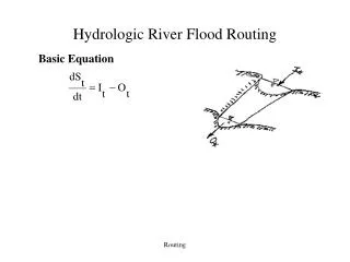
Hydrologic River Flood Routing Basic Equation Routing
Muskingum Method • For a non-uniform flow, Stf(Ot) • Because It=f(y1)and Ot= f(y2). Therefore, St=f(It,Ot). • Prism storage = f(Ot); Wedge storage = f(It, Ot). • Assume: Prism storage = KOt; Wedge storage = XK (It – Ot) • Total storage volume at any time instant, t, is St = KOt + XK (It - Ot) = K [X It + (1 - X)Ot] where K = travel time of flood wave in a reach, [hrs]; X = weighting factor, 0 ~ 0.5 Routing
Continuity Equation in Difference Form • Referring to figure, the continuity equation in difference form can be expressed as Routing
Derivation of Muskingum Routing Equation • By Muskingum Model, at t = t2, S2 = K [X I2 + (1 - X)O2] at t = t1, S1 = K [X I1 + (1 - X)O1] • Substituting S1, S2 into thecontinuity equation and after some algebraic manipulations, one has O2 = Co I2 + C1 I1 + C2 O1 • Replacing subscript 2 by t +1 and 1 by t, the Muskingum routing equation is Ot+1 = Co It+1 + C1 It + C2 Ot, for t = 1, 2, … where ; ; C2 = 1 – Co – C1 Note: K and t must have the same unit. Routing
Muskingum Routing Procedure • Given (knowns): O1; I1, I2, …; t; K; X • Find (unknowns): O2, O3, O4, … • Procedure: (a) Calculate Co, C1, and C2 (b) Apply Ot+1 = Co It+1 + C1 It + C2 Otstarting from t=1, 2, … recursively. Routing
Muskingum Routing - Example Routing
Estimating Muskingum Parameters (1) Graphical Method: • Referring to the Muskingum Model, find X such that the plot of XIt+ (1-X)Ot vs St behaves almost nearly as a single value curve. The corresponding slope is K. Routing
Example (Graphical Method) Routing
Estimating Muskingum Parameters (2) • Gill’s Least Square Method (Gill, 1978, “Flood routing by Muskingum method”, J. of Hydrology, V.36) St = K[XIt+(1-X)Ot] = KX It+K(1-X)Ot = AIt+BOt where A = KX, B = K(1-X) • Model: St’ = So + A It + B Ot, t = 1, 2, …, n where St’ = cumulative relative storage at time t; So = initial storage of channel before flood • Use least squares method to solve for A and B and So. Then, K and X can be obtained as K = A + B, X = A / (A + B) Routing
Example (Gill’s Method) Routing
Estimating Muskingum Parameters (3) • Stephensen’s Least Squares Method (Stephensen, 1979, “Direct optimization of Muskingum routing coefficient, “ J. of Hydrology, V.41) • Ot+1 = Co It+1 + C1 It + C2 Ot, t = 1, 2, …, n-1 • Use least squares method to estimate the values of Co, C1 and C2 directly. (Does not guarantee satisfying Co + C1 + C2 = 1) • Alternatively, Co + C1 + C2 =1, C2 = 1 – (Co + C1) (Ot+1 - Ot) = Co (It+1 - Ot) + C1 (It - Ot), t = 1, 2, …, n ; Routing
Example (Stephensen Method) Routing
Disadvantages of Hydrologic Routing (1) Ignore the dynamic effect of flow; (2) Assume stage and storage is a single–valued function of discharge - implying flow is changing slowly with time. Routing
Nonlinear Muskingum Model • In some stream reaches, St and XIt + (1-X)Ot reveals pronounced nonlinear relation. • To accommodate the non-linearity, the Muskingum model can be modified as St = K[XIt + (1-X)Ot]m or St = K[XItp + (1-X)Otq] • Using the nonlinear relationship, the routing becomes more difficult. A procedure using state-variable technique was developed by Tung (1985) to perform channel routing using nonlinear Muskingum model. Routing
Muskingum Crest Segment Routing • Purposes: • solve for single outflow rate or • route only a segment of inflow hydrograph • Basis: for t =1, 2, … Since By substituting Ot into the routing equation for Ot+1 and, after some algebraic manipulations, one has From recursive substitution of outflow at one time in terms of that at the previous time, one could have where K1=C0, K2 = C0 C2 + C1; Ki = Ki-1 C2, i≥3 Routing
Distributed Flow Routing • Estimate flow rate or water surface elevation at different locations and time simultaneously, rather than separately at different locations, so that the unsteady, non-uniform nature of actual flow phenomena are more closely modeled. • Modeling of flow movement can be in 1-D, 2-D, or 3-D in space and in time, depending on the dominant flow velocity field to be modeled. Routing
Governing Eqs. For Flow Routing(Saint-Venant Equations) Routing